
For policymakers or individuals to increase wellbeing depends on them understanding what might influence or drive wellbeing. Subjective wellbeing may be influenced by a wide range of individual and societal factors. The relative importance of different drivers is likely to vary across countries and across different groups within society depending on their circumstances. The seven contributions below use ESS data to explore a number of potentially important drivers of wellbeing across European countries: work, gender, parenthood, migration, the environment, democratic government and cultural values.
Feeling balanced? Perceived work-life balance and working conditions in Europe
Satisfaction with work-life balance depends on working hours, autonomy and flexibility. Analysis of the European Social Survey (ESS) demonstrates how many of these factors – and hence feelings of work- life balance – vary systematically across different employment regimes in Europe.
Introduction
We focus here on an important aspect of wellbeing: work-life balance. Increasingly work-life balance has been identified as a key element of quality of work1 (e.g. Kalleberg, 2011) and quality of life (e.g Anderson et al., 2009; Eurofound, 2012) and has been identified as an important indicator in attempts to ‘move beyond GDP’ in assessing social and economic progress (e.g. Stiglitz, Sen and Fitoussi, 2009). Work-life balance has also become a critical issue in academic and policy debates in Europe (European Commission, 2008). Rising female employment, lone parenthood, falling fertility and an ageing population have all brought the issue of reconciling work and caring demands to the fore. Conflict between the demands of work and family life has been linked to poorer outcomes in marital relations and child development and also to lower job satisfaction, absenteeism and stress (Allen et al., 2000).
One prominent debate in this vein of research is the extent to which work-life balance is influenced by pressures from work and pressures from home (Gallie and Russell, 2009; Jacobs and Gerson, 2004). The literature on institutional variations in advanced capitalist societies draws our attention to ways in which the demands of work and family may be mediated by the forms of production and welfare regimes in these societies. Different countries organise work in different ways, both in terms of working time and the quality of work (Gallie, 2007). A large body of work has also shown variation in how countries organise supports for non-work activities like caring and measures to support the reconciliation of work and family life (Gornick and Meyers, 2003; Plantenga and Remery, 2005). A key advantage of the harmonised cross-country data in surveys such as the European Social Survey (ESS) is that the role of these institutional differences can be examined. The ESS has provided the basis for extensive analysis of the drivers and consequences of work-family conflict2 (see McGinnity and Whelan, 2009; McGinnity and Russell, 2013; Gallie, 2013b). Building on this work, we here address three linked research questions:
- How do working conditions vary across country groups?
- How is satisfaction with work-life balance related to conditions in the workplace, after accounting for demands and resources within the household?
- Does institutional variation in working conditions help us to understand cross-national differences in satisfaction with work-life balance?
Meet the authors
Helen Russel
Associate Research Professor, Economic and Social Research Institute, Dublin and Adjunct Professor at Trinity College Dublin, Ireland
Frances McGinnity
Senior Research Officer, Economic and Social Research Institute Dublin and Adjunct Associate Professor at Trinity College Dublin, Ireland
What is work-life balance?
Work-life balance focuses attention on how individuals integrate paid work with the rest of their life (McGinnity, 2014). Much research in the area is rooted in the notion of a conflict between roles, i.e that meeting demands in one domain makes it difficult to meet demands in another. Working conditions can play an important role in determining how easy it is to manage that conflict: the demands-resources model distinguishes between work role demands – which may contribute to work-life conflict – and resources, which are factors used to cope with demands and reduce work-life conflict (Voyandoff, 2005).
One way to measure work-life balance in surveys such as the ESS is to ask people directly how satisfied they are with the way in which they manage the conflicting demands of different aspects of their lives. This study uses the following measure of work-life balance, included in Rounds 3 (2006/2007), 5 (2010/2011) and 6 (2012/2013) of the ESS:
And how satisfied are you with the balance between the time you spend on your paid work and the time you spend on other aspects of your life?
One way to measure work-life balance in surveys such as the ESS is to
ask people directly how satisfied they are
with the way in which they manage the conflicting demands of different aspects of their lives
| Extremely dissatisfied | Extremely satisfied | |||||||||
| 00 | 01 | 02 | 03 | 04 | 05 | 06 | 07 | 08 | 09 | 10 |
This measure refers to the overall level of contentment with how one handles work and other life demands. It captures perceptions and evaluations of an unspecified level of balance rather than the level of balance itself (Drobnic, 2011). As with other subjective measures of wellbeing it will also be related to individual expectations and adaptation.
Exploring work-life balance cross-nationally using the ESS
A module of questions focusing on ‘Work, Family and Wellbeing’ was fielded as part of the ESS in Round 2 (2004/2005) and Round 5 (2010/2011). For further information on the development of the module and the topics covered see here:
The analysis that follows uses ESS Round 5 data from 18 countries3, focusing on EU countries and Norway, where most research has been done to develop typologies comparing institutional conditions. The analysis is restricted to employees of working age defined as 20-64 years. Analysis of work-life balance is restricted to those who are living with a partner to allow analysis of the role of household employment patterns in work-life balance, a key theme in the literature.4 The data is weighted using the European Labour Force Survey to be representative of the working-age population (see Gallie, 2013a: pp. 28-29 for details).
We draw on employment regime theory and previous empirical research on the nature of working conditions and welfare support across countries (Gallie, 2013a) to identify five country groupings or regimes across which to compare working conditions and work-life balance.
- Liberal: UK, Ireland
- Nordic: Denmark, Norway, Sweden, Finland
- Continental: Germany, Netherlands, Belgium
- Southern: Greece, Spain, Portugal
- Transition: Estonia, Poland, Hungary, Slovakia, Czech Republic, Slovenia
Gallie (2007, 2013a) suggests differences in the quality of work across countries are shaped by employment regimes. Groups of countries are identified based on the inclusiveness of their collective bargaining arrangements measured by union density and bargaining coverage. Inclusive regimes have both extensive bargaining coverage in the economy and high union density. Dualist regimes have high bargaining coverage but low union density while liberal regimes have low levels of inclusiveness on both measures. In terms of work conditions, inclusive regimes are argued to promote long-term investment in employees and protect vulnerable workers. In dualist regimes there is a sharp contrast between the working conditions of the core and periphery, while in liberal systems, work conditions will depend on market power. These categories are ‘ideal type’ characterisations and in empirical work Gallie and Zhou (2013) assess how far conditions of employment and workers’ experiences vary within and across these groupings, distinguishing between five clusters of countries. In terms of employment regime, the Nordic countries cluster in the inclusive group, the Southern countries and the Continental countries fall into the dualist group, while the UK, Ireland and the Transition countries appear in the liberal group.
Differences in working conditions across countries
Using the country groupings outlined above we examine key working conditions across different employment regimes (Table 1 and Figure 1).5 The pattern of paid working hours in different regimes varies by gender.6 Table 1 shows that paid working hours are highest for men in the Transition and Southern countries. Paid working hours for women are lowest in the Continental and Liberal regimes, where part-time work is common, and highest in the Nordic, Transition and Southern countries where a higher proportion of women work full-time.7
Job pressure shows little variation by country group, but job control and flexible scheduling (being able to decide own start/finish times) are significantly higher in Nordic and Continental countries compared with other countries. The proportion of individuals who feel their job is insecure is much lower in the Nordic and Continental countries. The proportion of employees who feel their health and safety is at risk is lowest in the Nordic countries and considerably higher in the Transition countries (see Figure 1).
Table 1: Working hours, job pressure and job control by country group
| Liberal | Nordic | Continental | Southern | Transition | |
|---|---|---|---|---|---|
| Working hours (weekly) Men | 41.7 | 41 | 41.5 | 42.9 | 45.1 |
| Working hours (weekly) Women | 32 | 36.2 | 32.6 | 38 | 41.1 |
| Job Pressure Index (Mean score 1 to 5) | 3.6 | 3.4 | 3.4 | 3.5 | 3.3 |
| Index of job control (Mean score 0 to 10) | 4.9 | 6.7 | 5.6 | 4.5 | 4.2 |
Data source: European Social Survey Round 5 (2010/2011). Data weighted by labour market weights (Gallie, 2013a).
Note: Base for analysis is all employees, 20-64 years.
The Job Pressure Index is a combined measure (1-5) based on two questions from ESS Round 5 (2010/2011):
G34 My job requires that I work very hard.
G35 I never seem to have enough time to get everything done in my job.
Responses coded from 1 ‘disagree strongly’ to 5 ‘agree strongly’.
The Index of Job Control (0-10) is a measure of how much an individual can influence the pace of their work and how they organize it, as well as policy decisions about the activities of the organization. It is measured using a combination of these three questions from ESS Round 5 (2010/2011):
Please say how much the management at your work allows/allowed you…
F27 …to decide how your own daily work is/was organised?
F28 …to influence policy decisions about the activities of the organisation?
F28a …to choose or change your pace of work?
| I have/had no influence | I have/had complete control | |||||||||
| 00 | 01 | 02 | 03 | 04 | 05 | 06 | 07 | 08 | 09 | 10 |
Figure 1: Schedule flexibility, job insecurity and health and safety risk at work by country group
Data source: European Social Survey Round 5 (2010/2011). Data weighted by labour market weights (Gallie, 2013a).
Note: Base for analysis is all employees, 20-64 years. Figures for job insecurity are % saying “not at all true/a little true” that “my job is secure”.
Satisfaction with work-life balance and working conditions
What are the implications of this variation in working conditions for work-life balance? We explore this relationship by estimating a series of linear regression models to identify what predicts individuals’ responses on the scale of satisfaction with work-life balance. The analytical strategy here is to examine, firstly, how working conditions are related to perceived work-life balance, and, secondly, how far any regime differences observed in satisfaction with work-life balance can be explained by these differences in working conditions. We first present findings on how satisfaction with work-life balance is related to working conditions.
When we estimate a model of factors associated with work-life balance (see Appendix Table A.1), we find working hours are very strongly associated: those who work longer hours are much less satisfied with the balance between work and family life. Employer-driven flexibility, in particular working overtime at short notice, but also working unsocial hours like evenings, nights and weekends, reduces satisfaction with work-life balance. Employee control over start and finish times has a positive impact on satisfaction with work-life balance, albeit modest.
Work pressure has a very strong, significant association with perceived work-life balance: higher pressure at work is associated with lower satisfaction with work-life balance. Conversely, the model also shows that job control increases satisfaction with work-life balance, as found by Fagan and Walthery (2011). Having supportive colleagues is another resource which increases satisfaction. A final current job-related factor is job insecurity, which reduces satisfaction with work-life balance.
The full model also shows that family factors such as having a child under 6 decreases satisfaction with work-life balance among employees, while having a partner who works part-time significantly increases satisfaction. However, total number of children and total hours of housework undertaken by the respondent and their partner have no significant effect.
High satisfaction with work-life balance
in the Nordic countries is related to differences in working hours and better working conditions
Satisfaction with work-life balance and employment regime
How much does work-life balance vary across employment regimes and what role do family factors, working hours and working conditions play in understanding these regime differences? Figure 2 presents results from a series of nested regression models designed to examine this. Five successive regression models were run into which additional groups of predictor variables were added to the previous model to try and explain more of the variance observed in work-life balance across the five ESS country groupings representing different employment regimes. Results from Model 1 show that without taking account of any other factors, regime differences in satisfaction with work-life balance are significant but not large. Satisfaction with work-life balance is highest in the Nordic countries, followed by Continental and Liberal countries (Model 1). Satisfaction is lowest in Transition and Southern group countries (these are not significantly different from each other). Controlling for demographic factors (Model 2) and family (Model 3) makes no difference to regime patterns. We saw previously that paid working hours are highly salient for work-life balance: controlling for differences in working hours brings work-life balance satisfaction in Liberal countries to the same level as the Transition countries, and reduces the Nordic and Continental countries’ advantage (Model 4). Adding other working conditions halves the Nordic difference, suggesting higher job resources and lower demands account for much of the higher satisfaction observed in these countries (Model 5). The proportion of the total variation in satisfaction with work-life balance accounted for by different groups of factors (regime, demographic, family, working hours and other working conditions) is available in Appendix Table A.2.
Figure 2: Satisfaction with work-life balance by country group
Data source: European Social Survey Round 5 (2010/2011). Data weighted by labour market weights (Gallie, 2013a).
Note: Regression coefficients showing difference in work-life balance relative to the Transition countries (reference category), after controlling for demographic, family and working conditions. See Appendix Table A.1 for details of variables included in each model. Base for analysis is all employees, 20-64 years, living with partner.
Conclusion
Using data from the ESS module on ‘Work, Family and Wellbeing’, we find that satisfaction with work-life balance is strongly associated with working hours, autonomy, flexibility, and working unsocial hours, and that many of these factors vary systematically across employment regimes. We also find the satisfaction with work-life balance is higher among Nordic and Continental countries compared with other parts of Europe. Analysis suggests that this is related to differences in working hours and better working conditions in these countries. Wellbeing differences across the different country groupings or regimes are much reduced when we account for these differences. Family demands are also significant but, compared with working conditions, explain less of the overall variation in satisfaction with work-family balance and cross-national variation in this.
The analysis of work-balance presented here provides only a partial exploration of wellbeing. One enduring limitation of the concept of work-life balance is that, by definition, it only focuses on those in employment; other groups with lower than average wellbeing, like the unemployed and long-term sick, are not included in the analysis. Another limitation is that the focus here is on current wellbeing and it is not possible to account for any consequences that different levels of current work-life balance may have for future wellbeing, for example, as regards family formation or career development (McGinnity, 2014).
Nevertheless, there are important insights to be gained from an examination of work-life balance in cross-national perspective as made possible by the ESS. The findings suggest some clear lessons for policymakers and/or employers seeking to promote work-life balance. For example: ensuring predictable working hours that are not too long, facilitating employee autonomy, the ability to decide start/finish times and working during the standard working week, are all measures likely to enhance work-life balance.
The analysis presented here draws on two studies using data from the ESS ‘Work, Family and Wellbeing’ module:
McGinnity, F. and Russell, H. (in press)
‘Work-life Balance, Working Conditions and the Great Recession’. In: O’Riain, S., Flaherty, E., Ciccia, R., Behling, F. (ed) The Changing Worlds and Workplaces of Capitalism. Basingstoke: Palgrave Macmillan.
McGinnity, F. and Russell, H. (2013)
‘Work-family Conflict and Economic Change’. In: Gallie, D. (ed). Economic Crisis, Quality of Work and Social Integration: The European Experience. Oxford: Oxford University Press, pp. 169-194.
These studies also make use of the time series element of ESS data (the ‘Work, Family and Wellbeing’ module was fielded in Round 2 (2004/2005) and Round 5 (2010/2011)) to examine how recessionary factors, such as deteriorating work conditions and firm-level difficulties, are associated with lower satisfaction with work-life balance and higher levels of work to family conflict.
Allen, T., Herst, D., Bruck, C., Sutton, M. (2000)
‘Consequences Associated with Work-to-Family Conflict: A Review and Agenda for Future Research’. Journal of Occupational Health Psychology, 5, pp. 278-308.
Anderson, R., Mikulic, B., Vermeylen, G., Lyly-Yrjanainen, M., Zigante, V. (2009)
Second European Quality of Life Survey: Overview. Luxembourg, Eurofound.
Eurofound (2012)
Working time and work–life balance in a life course perspective: A report based on the fifth European Working Conditions Survey. Dublin, Eurofound.
European Commission (2008)
Commission improves work-life balance for millions with longer and better maternity leave. Press release [online] issued 3 October 2007.
Drobnic, S. (2011) ‘Introduction: Job Quality and Work-life balance’. In: Drobnic, S. and Guillen, A. (ed) Work-life Balance in Europe: The Role of Job Quality. Basingstoke: Palgrave Macmillan, pp. 1-16.
Fagan, C. and Walthery, P. (2011)
‘Job Quality and the Perceived Work-Life Balance fit between Work Hours and Personal Commitments: A Comparison of Parents and Older Workers in Europe’. In: Drobnic, S. and Guillen, A. (ed) Work-life Balance in Europe: The Role of Job Quality. Basingstoke: Palgrave Macmillan, pp. 69-94.
Gallie, D. (2013a)
‘Economic Crisis, the Quality of Work and Social Integration: Issues and Context’. In: Gallie, D. (ed) Economic Crisis, Quality of Work and Social Integration: The European Experience. Oxford: Oxford University Press, pp. 1-29.
Gallie, D. (2013b)
Economic Crisis, Quality of Work and Social Integration: Topline Results from Rounds 2 and 5 of the European Social Survey. London: Centre for Comparative Social Surveys.
Gallie, D. (2007)
‘Production Regimes, Employment Regimes and the Quality of Work’. In: Gallie, D. (ed) Employment Regimes and the Quality of Work. Oxford: Oxford University Press, pp. 1-34.
Gallie, D. and Zhou, Y. (2013)
‘Job Control, Work Intensity, and Work Stress’. In: Gallie, D. (ed) Economic Crisis, Quality of Work and Social Integration: The European Experience. Oxford: Oxford University Press, pp. 115-141.
Gallie, D. and Russell, H. (2009)
‘Work–family conflict and working conditions in Western Europe’. In: Social Indicators Research, 93(3), pp. 445–467.
Gornick, J. C. and Meyers, M.K. (2003)
Families That Work – Policies for Reconciling Parenthood and Employment. New York: Russell Sage Foundation.
Jacobs, J. A. and Gerson, K. (2004)
The Time Divide: Work, Family and Gender Inequality. Massachusetts: Harvard University Press.
Kalleberg, A. (2011)
Good Jobs, Bad Jobs : The Rise of Polarized and Precarious Employment Systems in the United States, 1970s to 2000s’. New York: Russell Sage Foundation.
McGinnity, F. (2014)
‘Work-life Conflict in Europe’. In: Michalos, A.C. (ed) Encyclopedia of Quality of Life and Well-Being Research. Dordrecht: Springer, pp. 7233-7236.
McGinnity, F. and Russell, H. (2013)
‘Work-family Conflict and Economic Change’. In: Gallie, D. (ed). Economic Crisis, Quality of Work and Social Integration: The European Experience. Oxford: Oxford University Press, pp. 169-194.
McGinnity, F. and Whelan, C.T. (2009)
‘Reconciling work and family life. Evidence from the European Social Survey’. Social Indicators Research, 93(3), pp. 433–445.
Plantenga, J. and Remery, C. (2005)
Reconciliation of work and private life: A comparative review of thirty European Countries. Luxembourg: Office for the Official Publications of the European Communities.
Stiglitz, J. E., Sen, A., Fitoussi, J. (2009)
Report by the Commission on the Measurement of Economic Performance and Social Progress.
Voyandoff, P. (2005)
‘Toward a Conceptualization of Perceived Work-Family Fit and Balance: A Demands and Resources Approach’. Journal of Marriage and Family, 67, pp. 822-836.
Modelling satisfaction with work-life balance
Linear regression was used to model the relative influence of different work and family characteristics on satisfaction with work-life balance. Positive coefficients indicate a positive effect on work- life balance, controlling for other factors included in the model, whilst negative coefficients indicate a negative effect on work-life balance.
Table A.1: Linear regression (dependent variable is satisfaction with work-life balance (0 to 10)), selected results
| B | Standardised coefficient | Sig | ||
|---|---|---|---|---|
| Regime Ref: Transition | Nordic | 0.270 | 0.061 | 0.000 |
| Liberal | 0.136 | 0.021 | 0.139 | |
| Southern | 0.122 | 0.019 | 0.166 | |
| Continental | 0.173 | 0.037 | 0.019 | |
| Demographic | Female | -0.193 | -0.048 | 0.000 |
| Age | 0.008 | 0.042 | 0.001 | |
| Family | No. of own children in household, any age | 0.008 | 0.004 | 0.733 |
| Any child under 6 years | -0.172 | -0.036 | 0.009 | |
| Ref: Partner 30-40hrs paid work | Partner not in paid work | 0.025 | 0.005 | 0.748 |
| Partner 1- 29 hrs paid work | 0.244 | 0.034 | 0.007 | |
| Partner over 40 hrs paid work | 0.022 | 0.004 | 0.753 | |
| Partner works unsocial hours | -0.028 | -0.024 | 0.164 | |
| Total housework hours (log) | 0.024 | 0.008 | 0.552 | |
| Work hours | Working hours (usual) | -0.037 | -0.186 | 0.000 |
| Other work conditions | Work evenings or nights (at least once a week) | -0.159 | -0.033 | 0.014 |
| Work overtime, short notice (at least once a week) | -0.504 | -0.094 | 0.000 | |
| Work weekends (at least several times per month) | -0.152 | -0.034 | 0.008 | |
| Can decide start/finish times (quite or very true) | 0.145 | 0.032 | 0.012 | |
| Job Pressure Index | -0.365 | -0.154 | 0.000 | |
| Health/safety at risk (quite or very true) | -0.471 | -0.091 | 0.000 | |
| Job control Index | 0.093 | 0.123 | 0.000 | |
| Support from colleagues | 0.489 | 0.097 | 0.000 | |
| Insecure about job | -0.360 | -0.083 | 0.000 | |
| (Constant) | 8.121 | 0.000 | ||
Data source: ESS Round 5 (2010/2011). Data weighted by labour market weights (Gallie, 2013a)
Note: Pooled analysis for 18 countries. Base for analysis is employees, 20-64 years, living with partner.
Explaining differences in work-life balance across employment regimes
Table A.2 shows the proportion of the variance in satisfaction with work-life balance scores that is explained by the different groups of explanatory variables when these are included in a series of nested linear regression models taking satisfaction with work-life balance (0-10) as the dependent variable. The variables included in each model are as shown in Table A.1. Family demands/resources explain a relatively low proportion of the variance in satisfaction. The low explanatory power of ‘family’ may arise because family borders are more permeable than work boundaries, which means that, for example, housework time is adjusted to fit in with work demands. Family demands may also be less well captured by the measures included; there is no measure of care for dependent adults for example. Work demands and resources are stronger predictors of satisfaction, especially working hours (5% of variance), and factors such as job pressure, job control (an additional 9% of variance).
Table A.2: Proportion of variance explained by groups of explanatory variables
| % Unique Variance Explained | As % of total variance explained | ||
|---|---|---|---|
| Model 1 | Regime | 2.3 | 13.2 |
| Model 2 | Sex and Age | 0.6 | 3.5 |
| Model 3 | Family | 0.3 | 1.8 |
| Model 4 | Paid working hours | 4.8 | 27.7 |
| Model 5 | Working Conditions | 9.2 | 53.8 |
| Total Variance Explained | 17.2 | 100 | |
| Variance Unexplained | 82.8 | ||
Data source: ESS Round 5 (2010/2011). Data weighted by labour market weights (Gallie, 2013a).
Note: Pooled analysis for 18 countries. Base for analysis is employees, 20-64 years, living with partner. The proportion of variance explained comes from the adjusted R-squared from a series of nested models. It represents the additional variance explained when each set of variables is added to the model in the order outlined in the table. See Table A.1 for further details of individual variables.
- ‘Quality of work’ is the sense of what constitutes a ‘good’ or ‘decent’ job for workers.
- See McGinnity and Whelan (2009) for a discussion of how far the concepts of work-family conflict and work-life balance overlap and how they have been measured.
- The 18 countries are those that fielded both Round 5 and Round 2 of the ESS and for which labour market weights were constructed (Gallie, 2013a). Of the available EU countries France was later excluded from our analysis due to uncertainty on where it should be placed in terms of employment regimes, and to missing information on some key variables. Norway was included with the EU countries because it is seen as a key exemplar of the Nordic employment regime.
- Analysis is based on a sample of 20,734 employees aged 20-64 and 13,370 employees living in couples.
- We do not examine here whether differences between groups of workers (e.g. high and low skilled) will vary across regimes but see Gallie and Zhou (2013). Working conditions may also vary between countries within regimes; the focus here is on variation between regimes.
- Working hours were top coded at 80 hours, following convention. Working hours tend to be longer among the self-employed, who are excluded from the current analysis.
- There is significant variation in women’s working hours within the Nordic group and the Southern group, see:
Gender inequalities and depression in Europe
Analysis of European Social Survey (ESS) data finds that more gender-equal societies promote better mental health among both men and women and reduce the gender gap in depressive symptoms.
Introduction
Mental health is an important component of wellbeing. Women are around twice as likely to report depressive symptoms and major depression as men (Van de Velde et al., 2010). However, this gender gap is not observed in all countries (Hopcroft and Bradley, 2007; Van de Velde et al., 2013) and also varies across the life span (Ferrari et al., 2013; McDowell et al., 2014).
Cross-national variation leads health sociologists to consider gender inequality as a potentially important culprit behind the higher incidence of depression in women. Because depression, lack of control, and powerlessness are related, gender stratification theory leads us to expect a substantial gender gap in depression in more gender-unequal societies.
Gender inequality relates, on the one hand, to the extent to which women and men who are otherwise social equals are unequal in their access to the scarce and valued resources of their society (Chafetz, 1984; Van de Velde et al., 2013). It additionally implies the unequal ability to define one’s goals and act upon them (Kabeer, 1999). Together, resources and agency constitute what Sen (1985) refers to as capabilities: the potential of men and women to live the lives they want to. When the failure to achieve one’s goals reflects some deep-seated constraint on the ability to choose, it can be taken as a manifestation of disempowerment. Because depression, lack of control, and powerlessness are related, a gender stratification theory leads us to expect a substantial gender gap in depression in gender-unequal societies.
However, the exact relationship between gender inequality and the gender gap in depression remains little understood. There have been only a handful of studies exploring this relationship empirically (Chen et al., 2005; Hopcroft and Bradley, 2007; McLaughlin, 2011; Seedat et al., 2009; Van de Velde et al., 2013) and their findings are inconsistent. In this contribution we seek to clarify the relationship between gender inequality and the gender gap in depression by combining gender stratification theory with a life course perspective, examining how the relationship between gender and depression varies with age.
We first outline the different theoretical perspectives on how age, gender and depression may be related before going on to present the results of an empirical exploration of this relationship using cross-national data from the European Social Survey (ESS).
Meet the authors
Piet Bracke
Professor of Sociology and Head of Health and Demographic Research (HeDeRa), Ghent University, Belgium
Rozemarijn Dereuddre
PhD Student, Ghent University, Belgium
Sarah Van de Velde
Postdoctoral Fellow, Research Foundation Flanders (FWO) and Ghent University, Belgium
Age, gender and depression
There are three competing theories as to how the gender gap in depression may vary across the life course, each with different implications for how we might also expect the gender gap to vary across countries depending on the level of gender inequality.
The gender gap in depression during the reproductive years
Part of the interest in gender differences in depression across age is related to the hypothesis that sex differences in endocrine physiology are involved (Cairney and Wade, 2002) with an onset of a gender gap in depression related to hormonal changes associated with puberty and a narrowing of the gender gap after the end of the reproductive life stage. Empirical findings are rather inconsistent and may vary depending on the social context, but in general this hypothesis leads us to expect a gender gap in depression that weakens after the reproductive years irrespective of social conditions i.e. regardless of the level of gender equality or inequality in a country (Figure 1).
Most studies find that a gender gap in depression is ubiquitous across all age groups after adolescence (Angst et al., 2002; Kuehner, 2003; Piccinelli and Wilkinson, 2000; Wade, Cairney and Pevalin, 2002) but there is mixed evidence regarding the trajectory of the gender gap throughout the reproductive years. Some studies report a widening of the gender gap during the reproductive years (Grigoriadis and Robinson, 2007) while other studies report smaller gender gaps in middle adulthood (Cairney and Wade, 2002; Mirowsky and Ross, 1992; Missinne et al., 2014).
As a substantial part of gender stratification encompasses a gendered organization of reproductive activities (Chafetz, 1988), we might expect a more pronounced gender gap in depression during the reproductive years in gender unequal societies. However, we also have to keep in mind that there are indications that biological differences between women and men can more freely manifest themselves in the absence of social constraints (Schmitt, 2014; Schmitt et al., 2008). This would bring us to expect more pronounced gender differences in depression during the reproductive years in gender equal societies.
For the present research question, it suffices to note that, in contrast to some of the other theories presented here, hormonal theories lead us to expect gender differences in depression to decrease in older age in all cases.
Figure 1: Depression by age and gender: Hormonal theory
Note: Stylised representation of relationship for illustrative purposes.
Age graded status and cumulative disadvantage
The lack of evidence for a simple hormonal model of depression in women (Kuehner, 2003) leads some scholars to stress the gendered impact on depression of social statuses related to various life stages. There are two possibilities.
The first relates age differences in depression to the age-structured organization of statuses and roles (Clarke et al, 2011; Mirowsky, 1996; Mirowsky and Ross, 1992). This age graded status composition perspective assumes that the relationship between age and depression is best explained by life stage-related social positions – such as marriage and employment – that are associated with mental health benefits and disadvantages (Clarke et al., 2011; Mirowsky, 1996; Mirowsky and Ross, 1992) (Figure 2a and Figure 2b). Different take up of these social positions by men and women between countries may explain the cross-national variation observed in the depression gender gap. Age, gender, and country differences in depression should, however, disappear after controlling for these life stage differences.
Figure 2a: Employment by age and gender: Age graded status composition theory
Data source: ESS Round 3 (2006/2007) and Round 6 (2012/2013). Design weights applied.
Note: Base for analysis is all respondents in employment.
Figure 2b: Marriage by age and gender: Age graded status composition theory
Data source: ESS Round 3 (2006/2007) and Round 6 (2012/2013). Design weights applied.
Note: Base for analysis is all married respondents.
The second possibility, cumulative disadvantage theory (CAD) (Dannefer, 2003), stresses the path dependence of transitions in and out of work and family-related roles and their advantages and disadvantages for mental health. CAD theory suggests that the association between disadvantage and depression strengthens as life unfolds (Figure 3). Both the incidence and duration of social deprivation and traumas, as well as the interaction between different forms of deprivation and trauma, accumulate across the life course, and result in more mental health problems as people age (George, 2014, Stansfeld et al., 2011).
Figure 3: Depression by age and gender: Cumulative disadvantage theory
Note: Stylised representation of relationship for illustrative purposes.
Combining CAD theory and gender stratification theory leads us to expect growing gender differences in depression with older age as any negative effects resulting from women’s relatively disadvantaged position accumulate. This widening gender gap will be particularly prominent in more gender-unequal societies where women’s cumulative disadvantage is greater. These accumulation processes surpass the individual occupancy of social positions and their mental health effects, and we expect to observe a gender gap of varying size across countries, even after taking individual differences in age graded status occupancy into account (Figure 4).
Combining cumulative disadvantage and gender stratification theories leads us to
expect growing gender differences in depression with older age
Figure 4: Depression by age and gender: Cumulative disadvantage theory in gender-equal and gender-unequal societies
Note: Stylised representation of relationship for illustrative purposes.
Maturation and adult development
Finally, some studies (George, 2014; Mirowsky and Ross, 1992) find that, after taking variation in social conditions and their accompanying losses and gains, and physical declines common in later life, into account, a negative relationship between age and depressive symptoms emerges. Maturation theory states that getting older comes with gaining life experience and people who have been confronted with social adversity learn to deal with it. There is some empirical evidence to support the idea that, with age, comes the capacity to make the best out of life (Chen and Miller, 2012; Schafer, Shippee and Ferraro, 2009; Mirowsky and Ross, 2001; Hatch, 2005).
In the context of this study, maturation theory – like hormonal theories – leads us to expects gender differences in depression to decline in older age as women (and men) in disadvantaged societies, or occupying disadvantaged positions, learn to cope with their condition and overcome their relative disadvantage (Figure 5).
Figure 5: Depression by age and gender: Maturation theory
Note: Stylised representation of relationship for illustrative purposes.
To test these competing theories, we combine data from ESS Round 3 (2006/2007) and Round 6 (2012/2013) and explore age differences in depressive symptoms between men and women across 28 countries.1 We focus on a subsample of respondents aged 21 to 90.2 Depression is measured using a shortened version of the Center for Epidemiologic Studies Depression Scale – CES-D8 (Radloff, 1977) included in the ESS rotating modules on ‘Personal and Social Wellbeing’3
Items constructing the CES-D8 scale
Please tell me how much of the time during the past week, …
… you felt depressed?
… you felt that everything you did was an effort?
… your sleep was restless?
… you were happy?
… you felt lonely?
… you enjoyed life?
… you felt sad?
… you could not get going?
Response categories are a 4-point scale (‘none or almost none of the time’; ‘some of the time’; ‘most of the time’; ‘almost all of the time’). Scores (0-3) for each of the CES-D8 items are combined to create an additive scale ranging from 0 to 24, with higher scores indicating a higher incidence of depressive symptoms.
The national level of gender inequality was assessed using the Global Gender Gap Index (GGI) 2006 and 2012 (World Economic Forum, 2013). We additionally control in our analysis for a range of individual socio-demographic variables, besides age and gender, including employment status, education, household income and marital status at the individual level as well as country’s income distribution as measured by the World Bank’s GINI index 2006 and 2012 (World Bank, 2014). See Appendix Table A.1 for more information on how all the variables have been coded and Appendix Table A.2 for how they are distributed across countries.
Multilevel models are used to investigate the effects of age, gender and the level of gender equality in society on the prevalence of depressive feelings across ESS countries. Analysis is conducted on the combined sample of cases from 2006 and 2012 controlling for between round changes in gender equality. The modelling strategy used and pooling data across two rounds allows us to explore variation in depression both across countries at a given point in time and within countries over time (though the over time results are not discussed here).4
Here we test three models. The first is a baseline model showing age-related gender differences in depression and how these vary across countries. The second model includes controls for individual work and family status allowing us to test the age graded status composition hypothesis. The third model includes country level variables and tests the impact of gender inequality in society on levels of depression among men and women.
Findings
The results of our modelling of ESS data are presented below. Full results can be found in the Appendix.
Age, gender and depression across countries
Analysis of ESS data confirms the well-known gender difference in depression, with women overall reporting higher mean scores on the depression scale. In addition, we notice substantial variation in the gender gap in depression between countries.5
Overall, the frequency and severity of depression symptoms among both men and women increases with age (see Appendix Table A.3, Model 1) with a more substantial increase beyond the age of 70 for men, and beyond 60 for women. As the age effect is more pronounced for women, this results in a more prominent gender difference in depression among those aged 61 and older. These findings provide evidence against the hormonal and maturation theories (which would predict a decline in depression and narrowing gender gap with age), and rather suggests that the gender gap in is related to social conditions. The relationship between age, gender and depressive symptoms found in the ESS data is visualised in Figure 6.
ESS data confirm the well-known gender difference in depression with
women reporting higher scores on the depression scale
Figure 6: Age differences in depressive symptoms among women and men
Data source: ESS Round 3 (2006/2007) and Round 6 (2012/2013). Design weights applied.
The impact of age graded social statuses
The next step in the analysis is to control for differences in social status which might explain variation in the incidence of depressive symptoms across the sample (see Appendix Table A.3, Model 2). Familiar differences in mental health among various work and family-related social categories are confirmed, with more severe depression symptoms among the unemployed, the sick and disabled, the retired and housekeepers (not shown in Appendix Table A.3). A higher income is associated with better mental health. Furthermore, we observe fewer depressive symptoms among the married and cohabiting, as well as among those with children below the age of 12 in the household. Interestingly, we notice only a minor reduction of the overall gender gap in depression, when these individual differences in work and family-related statuses are accounted for.
To evaluate the age graded status composition hypothesis, we look at the reduction of gender differences in depression across age categories after controlling for these work and family factors (comparing Model 1 and Model 2 in the Appendix Table A.3). A substantial reduction of the gender gap in depression among those aged 61 and older can be identified. Also, among those in middle adulthood a still significant, but smaller, reduction in the gender gap is observed.
The finding that gender differences in depression are to a certain extent related to the status composition of the various age categories provides evidence for the age graded model. Further, the fact that the reduction of the gender gap in depression after controlling for social status is most pronounced among older adults provides evidence in support of cumulative disadvantage theory (which predicts that the effect of social status increases with age as any negative effects accumulate).
The impact of gender stratification
Finally we consider the impact of gender inequality at the country level on depression and look at how the gap in depressive symptoms between men and women of different ages varies between more and less gender-unequal countries (Appendix Table A.3, Model 4).
Figure 7 shows how the incidence of depressive symptoms varies by age between men and women depending on whether the country is in the highest, middle or lowest tertile on gender equality according to the Global Gender Gap Index.6
Figure 7: Gender gap in depression by country-level gender inequality
Data source: ESS Round 3 (2006/2007) and Round 6 (2012/2013), World Economic Forum (2013) for GGI. Design weights applied to ESS data.
Overall, we notice a highly significant association between gender equality and depression; both women and men experience less depressive symptoms in more gender-equal countries. However, the positive effect of gender equality in reducing depression is more pronounced among women than men. This means that the gender gap in depression between men and women is smaller in more gender-equal countries than in less gender-equal countries.
Even in highly gender-equal countries, a significant gender gap does emerge among older adults; the result of a decline in depressive symptoms among men but not women between the ages of 50 and 70. However, the depression gap between men and women is less pronounced at all ages in more gender-equal countries compared with less gender-equal countries (and almost absent in young adults).
In countries where women face more unequal treatment, the lifelong accumulation of this disadvantage is more pronounced and the gender gap in depression which emerges with age greater. The finding confirms the complementarity of cumulative disadvantage and gender inequality theory in explaining gender differences in depression across countries and age categories.
Conclusion
Using ESS data on the incidence of depressive symptoms we have explored the relationship between age, gender and depression across different European countries. Consistent with a combination of gender stratification theory and cumulative disadvantage theory, we find that gendered opportunity structures impact the lives of women and men, and lead to gender differentiated mental health outcomes later in life.
These outcomes partially result from the age-specific occupancy of work and family-related social positions by women and men, but cannot be reduced to this. The level of gender inequality in society also has a role to play. This is an important observation. Most health sociological and social epidemiological studies focus on the individual social positions of women and men and, hence, underestimate the impact of gendered societal arrangements on depression. It is important to notice that less gender inequality goes hand in hand with better mental health for both women and men (though especially women). This has important implications for policymakers, suggesting the importance of policies to promote gender equality in different spheres including education, employment and politics.
As the CES-D8 is also part of Round 7 of the ESS (2014/2015), interested researchers will be able to investigate whether these findings can be replicated. Moreover, additional rounds of data on the prevalence of depressive symptoms among Europeans will provide opportunities to test whether any further evolution towards more gender-equal European societies results in a reduction or elimination of the gender gap in depression.
For further exploration of the gender gap in depression across Europe using ESS data, see the following:
Van de Velde, S., Huijts, T., Bracke, P., Bambra, C. (2013)
‘Macro‐level gender equality and depression in men and women in Europe’. Sociology of health & illness, 35(5), pp. 682-698.
Van de Velde, S., Bracke, P., Levecque, K. (2010)
‘Gender differences in depression in 23 European countries. Cross-national variation in the gender gap in depression’. Social Science & Medicine, 71(2), pp. 305-313.
Van de Velde, S., Bracke, P., Levecque, K., Meuleman, B. (2010)
‘Gender differences in depression in 25 European countries after eliminating measurement bias in the CES-D 8’. Social Science Research, 39(3), pp. 396-404.
Angst, J., Gamma, A., Gastpar, M., Lépine, J.P., Mendlewicz, J., Tylee, A. (2002)
‘Gender differences in depression’. European Archives of Psychiatry and Clinical Neuroscience, 252(5), pp. 201-209.
Cairney, J. and Wade, T.J. (2002)
‘The influence of age on gender differences in depression. Further population-based evidence on the relationship between menopause and the sex difference in depression’. Social Psychiatry and Psychiatric Epidemiology, 37(9), pp. 401-408.
Chafetz, J.S. (1984)
Sex and advantage: A comparative, macro-structural theory of sex stratification. Totowa (N.J.): Rowman & Allanheld.
Chafetz, J.S. (1988)
‘The gender division of labor and the reproduction of female disadvantage toward an integrated theory’. Journal of Family Issues, 9(1), pp. 108-131.
Chen, E. and Miller, G.E. (2012)
‘“Shift-and-Persist” strategies why low socioeconomic status isn’t always bad for health’. Perspectives on Psychological Science, 7(2), pp. 135-158.
Chen, Y.Y., Subramanian, S.V., Acevedo-Garcia, D., Kawachi, I. (2005)
‘Women’s status and depressive symptoms: A multilevel analysis’. Social Science & Medicine, 60(1), pp. 49-60.
Clarke, P., Marshall, V., House, J., Lantz, P. (2011)
‘The social structuring of mental health over the adult life course: Advancing theory in the sociology of aging’. Social Forces, 89(4), pp. 1287-1313.
Dannefer, D. (2003)
‘Cumulative advantage/disadvantage and the life course: Cross-fertilizing age and social science theory’. Journals of Gerontology Series B-Psychological Sciences and Social Sciences, 58(6), pp. S327-S337.
Dereuddre, R., Missinne, S., Buffel, V., Bracke, P. (2014)
‘Gender specific effects of financial and housework contributions on depression: A multi-actor study among three household types in Belgium’. Health Sociology Review, 23(2), pp. 78-90.
Fairbrother, M. (2013)
Two multilevel modeling techniques for analyzing comparative longitudinal survey datasets. University of Bristol.
Ferrari, A.J., Somerville, A.J., Baxter, A.J., Norman, R., Patten, S.B., Vos, T., Whiteford, H.A. (2013)
‘Global variation in the prevalence and incidence of major depressive disorder: A systematic review of the epidemiological literature’. Psychological Medicine, 43, pp. 471-481.
George, L.K. (2014)
‘Taking time seriously: A call to action in mental health research’. Journal of Health and Social Behavior, 55(3), pp. 251-264.
Grigoriadis, S. and Robinson, G.E. (2007)
‘Gender issues in depression’. Annals of Clinical Psychiatry, 19(4), pp. 247-255.
Hatch, S.L. (2005)
‘Conceptualizing and identifying cumulative adversity and protective resources: Implications for understanding health inequalities’. Journals of Gerontology Series B-Psychological Sciences and Social Sciences, 60(2), pp. 130-134.
Hopcroft, R.L. and Bradley, D.B. (2007)
‘The sex difference in depression across 29 countries’. Social Forces, 85(4), pp. 1483-1507.
Kabeer, N. (1999)
‘Resources, agency, achievements: Reflections on the measurement of women’s empowerment’. Development and Change, 30(3), pp. 435-464.
Kuehner, C. (2003)
‘Gender differences in unipolar depression: an update of epidemiological findings and possible explanations’. Acta Psychiatrica Scandinavica, 108(3), pp. 163-174.
McDowell, R.D., Ryan, A., Bunting, B.P., O’Neill, S.M., Alonso, J., Bruffaerts, R., Tomov, T. (2014) ‘Mood and anxiety disorders across the adult lifespan: A European perspective’. Psychological Medicine, 44(4), pp. 707-722.
McLaughlin, K.A. (2011)
‘The public health impact of major depression: A call for interdisciplinary prevention efforts’. Prevention Science, 12(4), pp. 361-371.
Mirowsky, J. and Ross, C.E. (1992)
‘Age and depression’. Journal of Health and Social Behavior, 33(3), pp. 187-205.
Mirowsky, J. (1996)
‘Age and the gender gap in depression’. Journal of Health and Social Behavior, 37(4), pp. 362-380.
Mirowsky, J. and Ross, C.E. (2001)
‘Age and the effect of economic hardship on depression’. Journal of Health and Social Behavior, 42(2), pp. 132-150.
Missinne, S., Vandeviver, C., Van de Velde, S., Bracke, P. (2014)
‘Measurement equivalence of the CES-D 8 depression-scale among the ageing population in eleven European countries’. Social Science Research, 46, pp. 38-47.
Piccinelli, M. and Wilkinson, G. (2000)
‘Gender differences in depression. Critical review’. The British Journal of Psychiatry, 177(6), pp. 486-492.
Radloff, L.S. (1977)
‘The CES-D scale: A self-report depression scale for research in the general population’. Applied Psychological Measurement, 1(3), pp. 385-401.
Schafer, M.H., Shippee, T.P., Ferraro, K.F. (2009)
‘When does disadvantage not accumulate? Toward a sociological conceptualization of resilience’. Schweizerische Zeitschrift für Soziologie, 35(2), pp. 231-251.
Schmitt, D.P. (2014)
‘The evolution of culturally-variable sex differences: Men and women are not always different, but when they are… it appears not to result from patriarchy or sex role socialization’. In: Weekes-Shackelford, V.A. and Shackelford, T.K. (ed) The Evolution of Sexuality. New York: Springer, pp. 221-256.
Schmitt, D.P., Realo, A., Voracek, M., Allik, J. (2008)
Why can’t a man be more like a woman? Sex differences in Big Five personality traits across 55 cultures’. Journal of Personality and Social Psychology, 94(1), pp. 168-182.
Seedat, S., Scott, K.M., Angermeyer, M.C., Berglund, P., Bromet, E.J., Brugha, T.S., Jin, R. (2009)
‘Cross-national associations between gender and mental disorders in the World Health Organization World Mental Health Surveys’. Archives of General Psychiatry, 66(7), pp. 785-795.
Sen, A.K. (1985)
Commodities and capabilities. Amsterdam: North-Holland.
Stansfeld, S.A., Clark, C., Rodgers, B., Caldwell, T., Power, C. (2011)
‘Repeated exposure to socioeconomic disadvantage and health selection as life course pathways to mid-life depressive and anxiety disorders’. Social Psychiatry and Psychiatric Epidemiology, 46(7), pp. 549-558.
Van de Velde, S., Bracke, P., Levecque, K., Meuleman, B. (2010)
‘Gender differences in depression in 25 European countries after eliminating measurement bias in the CES-D 8’. Social Science Research, 39(3), pp. 396-404.
Van de Velde, S., Bracke, P., Levecque, K. (2010)
‘Gender differences in depression in 23 European countries. Cross-national variation in the gender gap in depression’. Social Science & Medicine, 71(2), pp. 305-313.
Van de Velde, S., Huijts, T., Bracke, P., Bambra, C. (2013)
‘Macro-level gender equality and depression in men and women in Europe’. Sociology of Health & Illness, 35(5), pp. 682-698.
Wade, T.J., Cairney, J., Pevalin, D.J. (2002)
‘Emergence of gender differences in depression during adolescence: National panel results from three countries’. Journal of the American Academy of Child & Adolescent Psychiatry, 41(2), pp. 190-198.
World Bank (2014)
World development indicators: Distribution of income or consumption.
World Economic Forum (2013)
The global gender gap report 2013.
Table A.1: Coding applied to variables included in multivariate models
| Variable name | Categories | Number of items | Range |
|---|---|---|---|
| Micro-level variables | |||
| Depression symptoms (CESD-8) | 8 | 0-24 | |
| Years of education | 1 | 0-30 | |
| Gender | Men (Ref.) | ||
| Women | |||
| ESS round | 3 (Ref.) | ||
| 6 | |||
| Age | 21 – 30 (Ref.) | ||
| 31 – 40 | |||
| 41 – 50 | |||
| 51 – 60 | |||
| 61 – 70 | |||
| 71 – 80 | |||
| 81 – 90 | |||
| Employment status | Paid employment (Ref.) | ||
| Student | |||
| Unemployed | |||
| Permanently sick or disabled | |||
| Retired | |||
| Housekeeper | |||
| Other | |||
| EQ household income | <50% of the median equivalent income | ||
| 50-79% | |||
| 80-120% | |||
| ≥ 120% (Ref.) | |||
| Missing | |||
| Marital status | Married/civil union (Ref.) | ||
| Divorced or separated | |||
| Widowed | |||
| Single | |||
| Children aged below 12 | No (Ref.) | ||
| Yes | |||
| Macro-level variables | |||
| GINI | 1 | 0-100 | |
| Global Gender Gap Index (GGI) | 4 | 0-1 | |
Table A.2: Descriptive statistics of country characteristics
| GINI | GGI | CESD-8 | Years of education (mean) | Married | Employed | < 80% of country median income | Children below 12 vs. no children below 12 | ||||||||||||
|---|---|---|---|---|---|---|---|---|---|---|---|---|---|---|---|---|---|---|---|
| 2006 | 2012 | Mean | 2006 | 2012 | Mean | 2006 | 2012 | Mean | 2006 | 2012 | 2006 | 2012 | 2006 | 2012 | 2006s | 2012 | 2006 | 2012 | |
| Albania | 33 | 34.5 | 33.8 | 0.66 | 0.67 | 0.66 | – | 9.77 | 9.77 | – | 10.6 | – | 0.76 | – | 0.3 | – | 0.39 | – | 0.34 |
| Austria | 25.3 | 27.6 | 26.5 | 0.7 | 0.74 | 0.72 | 5.53 | – | 5.53 | 12.5 | – | 0.52 | – | 0.6 | – | 0.23 | – | 0.2 | – |
| Belgium | 27.8 | 26.6 | 27.2 | 0.71 | 0.77 | 0.74 | 5.44 | 5.3 | 5.36 | 12.4 | 13.1 | 0.67 | 0.55 | 0.53 | 0.53 | 0.29 | 0.23 | 0.23 | 0.22 |
| Bulgaria | 31.2 | 33.6 | 32.4 | 0.69 | 0.7 | 0.69 | 8.19 | 7.28 | 7.61 | 11.2 | 11.5 | 0.64 | 0.54 | 0.44 | 0.43 | 0.23 | 0.35 | 0.19 | 0.17 |
| Cyprus | 28.8 | 31 | 29.9 | 0.64 | 0.67 | 0.66 | 5.31 | 5.68 | 5.5 | 11.3 | 12 | 0.7 | 0.64 | 0.54 | 0.5 | 0.22 | 0.34 | 0.22 | 0.2 |
| Czech Republic | 25.3 | 24.9 | 25.1 | 0.67 | 0.68 | 0.67 | – | 7.21 | 7.21 | – | 13 | – | 0.57 | – | 0.58 | – | 0.19 | – | |
| Denmark | 23.7 | 28.1 | 25.9 | 0.75 | 0.78 | 0.76 | 5.76 | 4.47 | 4.62 | 13.2 | 13.7 | 0.6 | 0.59 | 0.59 | 0.67 | 0.29 | 0.22 | 0.25 | 0.26 |
| Estonia | 33.1 | 32.5 | 32.8 | 0.69 | 0.7 | 0.7 | 6.91 | 6.71 | 6.79 | 12.4 | 12.8 | 0.48 | 0.45 | 0.6 | 0.54 | 0.21 | 0.27 | 0.2 | 0.2 |
| Finland | 25.9 | 25.9 | 25.9 | 0.8 | 0.85 | 0.82 | 4.98 | 4.67 | 4.81 | 12.5 | 13.3 | 0.55 | 0.53 | 0.55 | 0.53 | 0.32 | 0.29 | 0.21 | 0.19 |
| France | 27.3 | 30.5 | 28.9 | 0.65 | 0.7 | 0.68 | 5.61 | 5.72 | 5.67 | 12.5 | 12.4 | 0.55 | 0.5 | 0.55 | 0.49 | 0.3 | 0.27 | 0.28 | 0.21 |
| Germany | 26.8 | 28.3 | 27.6 | 0.75 | 0.76 | 0.76 | 6.12 | 5.61 | 5.86 | 13.3 | 14,0 | 0.58 | 0.6 | 0.49 | 0.52 | 0.27 | 0.26 | 0.17 | 0.17 |
| Hungary | 33.3 | 26.9 | 30.1 | 0.67 | 0.67 | 0.67 | 8.76 | 8.06 | 8.37 | 11.7 | 12.4 | 0.54 | 0.48 | 0.42 | 0.49 | 0.21 | 0.22 | 0.19 | 0.19 |
| Iceland | 26.3 | 24 | 25.2 | 0.78 | 0.86 | 0.82 | – | 4.44 | 4.44 | – | 15,0 | – | 0.48 | – | 0.61 | – | 0.33 | – | 0.31 |
| Ireland | 31.9 | 29.9 | 30.9 | 0.73 | 0.78 | 0.76 | 4.83 | 4.72 | 4.76 | 12.7 | 14,0 | 0.53 | 0.53 | 0.52 | 0.42 | 0.31 | 0.24 | 0.29 | 0.26 |
| Israel | 37.8 | 37.6 | 37.7 | 0.69 | 0.7 | 0.69 | – | 5.88 | 5.88 | – | 13.6 | – | 0.68 | – | 0.54 | – | 0.27 | – | 0.32 |
| Italy | 32.1 | 31.9 | 32 | 0.65 | 0.67 | 0.66 | – | 6.61 | 6.61 | – | 12.5 | – | 0.57 | – | 0.53 | – | 0.25 | – | 0.19 |
| Latvia | 38.9 | 35.7 | 37.3 | 0.7 | 0.74 | 0.72 | 8.23 | – | 8.23 | 11.8 | – | 0.47 | – | 0.58 | – | 0.34 | – | 0.2 | – |
| Lithuania | 35,0 | 32,0 | 33.5 | 0.71 | 0.72 | 0.71 | – | 7.41 | 7.41 | – | 12.7 | – | 0.53 | – | 0.54 | – | 0.24 | – | 0.19 |
| Netherlands | 26.4 | 25.4 | 25.9 | 0.73 | 0.77 | 0.75 | 5.34 | 5.01 | 5.18 | 13.1 | 13.6 | 0.54 | 0.54 | 0.51 | 0.5 | 0.33 | 0.28 | 0.22 | 0.19 |
| Norway | 29.2 | 22.6 | 25.9 | 0.8 | 0.84 | 0.82 | 4.2 | 3.86 | 4.04 | 13.6 | 13.3 | 0.57 | 0.55 | 0.66 | 0.66 | 0.35 | 0.27 | 0.26 | 0.26 |
| Poland | 33.3 | 30.9 | 32.1 | 0.68 | 0.7 | 0.69 | 6.86 | 5.87 | 6.34 | 11.7 | 12.5 | 0.63 | 0.64 | 0.5 | 0.53 | 0.32 | 0.26 | 0.29 | 0.26 |
| Portugal | 37.7 | 34.5 | 36.1 | 0.69 | 0.71 | 0.7 | 7.87 | 6.98 | 7.43 | 7.1 | 7.9 | 0.6 | 0.52 | 0.48 | 0.4 | 0.18 | 0.17 | 0.21 | 0.18 |
| Romania | 33 | 33.2 | 33.1 | 0.68 | 0.69 | 0.68 | 7.5 | – | 7.5 | 10.7 | – | 0.68 | – | 0.4 | – | 0.33 | – | 0.22 | – |
| Russia | 42.1 | 42 | 42.1 | 0.68 | 0.7 | 0.69 | 8.23 | 7.44 | 7.83 | 12.2 | 13.1 | 0.49 | 0.47 | 0.55 | 0.61 | 0.38 | 0.24 | 0.2 | 0.2 |
| Slovakia | 28.1 | 25.3 | 26.7 | 0.68 | 0.68 | 0.68 | 7.46 | 6.99 | 7.21 | 12.6 | 13.1 | 0.66 | 0.58 | 0.57 | 0.5 | 0.22 | 0.16 | 0.26 | 0.17 |
| Slovenia | 23.7 | 23.7 | 23.7 | 0.67 | 0.71 | 0.69 | 5.87 | 4.73 | 5.34 | 11.8 | 12,0 | 0.69 | 0.54 | 0.46 | 0.45 | 0.27 | 0.24 | 0.21 | 0.2 |
| Spain | 31.9 | 35 | 33.5 | 0.73 | 0.73 | 0.73 | 5.67 | 6.28 | 5.98 | 11.7 | 12.3 | 0.62 | 0.58 | 0.57 | 0.46 | 0.22 | 0.34 | 0.22 | 0.23 |
| Sweden | 24 | 24.8 | 24.4 | 0.81 | 0.82 | 0.81 | 4.95 | 4.59 | 4.77 | 12.8 | 13.1 | 0.48 | 0.51 | 0.66 | 0.59 | 0.35 | 0.31 | 0.22 | 0.22 |
| Switzerland | 30.3 | 28.8 | 29.6 | 0.7 | 0.77 | 0.73 | 4.77 | 4.69 | 4.73 | 13.3 | 11.8 | 0.58 | 0.59 | 0.56 | 0.6 | 0.29 | 0.28 | 0.19 | 0.19 |
| Ukraine | 29.7 | 25.6 | 27.7 | 0.68 | 0.69 | 0.68 | 8.86 | 8.25 | 8.54 | 11.6 | 12.5 | 0.58 | 0.54 | 0.43 | 0.43 | 0.24 | 0.22 | 0.21 | 0.22 |
| UK | 32.5 | 32.8 | 32.7 | 0.74 | 0.74 | 0.74 | 5.86 | 5.63 | 5.75 | 13.4 | 13.3 | 0.53 | 0.52 | 0.53 | 0.48 | 0.34 | 0.33 | 0.23 | 0.2 |
Data source: ESS Round 3 (2006/2007) and Round 6 (2012/2013), World Bank (2014) for GINI, World Economic Forum (2013) for GGI. Design weights applied to ESS data.
Table A.3: Multilevel model of depressive symptoms (score on CES-D8 (0 to 24)) regressed on respondents’ social positions and countries’ level of gender equality
| Intercept-only model | Model 1 | Model 2 | Model 3 | Model 4 | ||||||
|---|---|---|---|---|---|---|---|---|---|---|
| β | s.e. | β | s.e. | β | s.e. | β | s.e. | β | s.e. | |
| Intercept | 6.158 | 0.244*** | 5.376 | 0.171*** | 4.346 | 0.176*** | 4.329 | 0.146*** | 4.372 | 0.145*** |
| Micro level variables | ||||||||||
| Woman | 0.459 | 0.103*** | 0.543 | 0.099*** | 0.524 | 0.100*** | 0.567 | 0.097*** | ||
| ESS round 2012 | -0.371 | 0.090*** | -0.371 | 0.080*** | -0.425 | 0.134** | -0.415 | 0.136** | ||
| Age (ref. = aged 21-30) | ||||||||||
| 31 – 40 | 0.208 | 0.091* | 0.591 | 0.093*** | 0.591 | 0.093*** | 0.557 | 0.087*** | ||
| 41 – 50 | 0.449 | 0.137** | 0.733 | 0.127*** | 0.734 | 0.127*** | 0.696 | 0.117*** | ||
| 51 – 60 | 0.763 | 0.187*** | 0.814 | 0.163*** | 0.815 | 0.163*** | 0.776 | 0.147*** | ||
| 61 – 70 | 0.604 | 0.250* | 0.338 | 0.209 | 0.339 | 0.208 | 0.366 | 0.174* | ||
| 71 – 80 | 1.162 | 0.282*** | 0.579 | 0.224** | 0.581 | 0.223** | 0.612 | 0.177*** | ||
| 81 – 90 | 1.961 | 0.266*** | 1.037 | 0.208*** | 1.038 | 0.208*** | 1.164 | 0.176*** | ||
| Age*Women | ||||||||||
| 31 – 40*Woman | 0.069 | 0.122 | -0.061 | 0.113 | -0.061 | 0.113 | -0.073 | 0.104 | ||
| 41 – 50*Woman | 0.228 | 0.099* | 0.003 | 0.094 | 0.003 | 0.094 | -0.032 | 0.096 | ||
| 51 – 60*Woman | 0.323 | 0.139* | 0.048 | 0.139 | 0.048 | 0.139 | 0.009 | 0.14 | ||
| 61 – 70*Woman | 0.866 | 0.139*** | 0.353 | 0.148* | 0.354 | 0.147* | 0.291 | 0.158 | ||
| 71 – 80*Woman | 1.244 | 0.139*** | 0.406 | 0.135** | 0.408 | 0.135** | 0.359 | 0.143* | ||
| 81 – 90*Woman | 1.045 | 0.279*** | -0.009 | 0.259 | -0.007 | 0.259 | -0.03 | 0.257 | ||
| Macro level variables | ||||||||||
| GINI | 0.081 | 0.035* | 0.081 | 0.036* | ||||||
| GGI | -13.116 | 3.969*** | -5.784 | 3.318 | ||||||
| Women*GGI | -4.269 | 1.121*** | -0.601 | 1.926 | ||||||
| Age*GGI | ||||||||||
| 31 – 40* GGI | -0.598 | 1.392 | ||||||||
| 41 – 50* GGI | -6.726 | 2.252** | ||||||||
| 51 – 60* GGI | -9.504 | 2.851*** | ||||||||
| 61 – 70* GGI | -14.164 | 3.843*** | ||||||||
| 71 – 80* GGI | -16.416 | 4.405*** | ||||||||
| 81 – 90* GGI | -17.537 | 4.470*** | ||||||||
| Change in GGI | 2.014 | 3.465 | 1.655 | 3.53 | ||||||
| Woman*Change in GGI | 0.449 | 1.604 | 0.26 | 1.6 | ||||||
| Age*Woman*GGI | ||||||||||
| 31 – 40*Woman*GGI | -4.725 | 2.083* | ||||||||
| 41 – 50*Woman*GGI | -2.187 | 1.662 | ||||||||
| 51 – 60*Woman*GGI | -1.929 | 2.532 | ||||||||
| 61 – 70*Woman*GGI | -4.925 | 2.633 | ||||||||
| 71 – 80*Woman*GGI | -7.376 | 2.850** | ||||||||
| 81 – 90*Woman*GGI | -11.352 | 3.733** | ||||||||
| Variance | ||||||||||
| Country | 1.747 | 0.387*** | 1.686 | 0.413*** | 1.51 | 0.351*** | 0.787 | 0.211*** | 0.765 | 0.206*** |
| Period*country | 0.144 | 0.038*** | 0.076 | 0.024** | 0.061 | 0.021** | 0.06 | 0.023** | 0.061 | 0.023** |
| Individual | 16.194 | 0.705*** | 15.563 | 0.604*** | 14.354 | 0.542*** | 14.354 | 0.542*** | 14.253 | 0.539*** |
| Random slope woman | 0.153 | 0.033*** | 0.13 | 0.032*** | 0.091 | 0.029** | 0.091 | 0.028** | ||
| -2*loglikelihood | 509594.663 | 506095.733 | 498883.932 | 498848.575 | 498225.486 | |||||
Data source: ESS Round 3 (2006/2007) and Round 6 (2012/2013), World Bank (2014) for GINI, World Economic Forum (2013) for GGI. Design weights applied to ESS data.
Note: * p < 0.05; ** p < 0.01; *** p < 0.001. Models 2, 3 and 4 control for years of education, employment status, equivalent household income, marital status and children aged below 12.
- All ESS countries from Rounds 3 and 6 are included, except for Kosovo (ESS6) because information on the Global Gender Gap Index (used in analysis) is currently not available.
- This gives a sample size of 40, 322 men and 48,832 women.
- Reliability of the CES-D8 scale is good (Cronbach’s alphamen = 0.816; Cronbach’s alphawomen = 0.847) and the validity of the inventory across gender, age groups, and European countries is confirmed (Missinne et al., 2014; Van de Velde et al., 2010).
- We follow the method suggested by Fairbrother (2013) and use a three-level model to take the clustering of the data in countries into account and to simultaneously model the within-country change between the two rounds. Individuals are nested within country-specific rounds 2006 and 2012, which are nested in countries. In other words, both the cross-sectional effects that explain between-country differences and the change effect that explains the within-country differences over time are modelled. Because several countries only participated in one wave, 53 country-specific rounds and 31 countries are included in the analyses. By including the change effect, we come to more reliable estimates of the cross-sectional effect, given the complex nature of our sample.
- For the intercept only model: βgender = 0.881, s.e. = 0.075, p < 0.001; u = 0.147, s.e. = 0.031, p < 0.001
- Lowest (most unequal) tertile: Albania, Hungary, Cyprus, Italy, France, Romania, Slovakia, France, Ukraine. Middle: Bulgaria, Poland, Slovenia, Portugal, Lithuania, Israel, Russia, Estonia, Austria, Latvia, Spain, Switzerland. Highest (most equal) tertile: Belgium, UK, Netherlands, Denmark, Germany, Ireland, Sweden, Finland, Iceland, Norway.
The positive effect of gender equality in reducing depression is more pronounced among women. This means
the gender gap in depression is smaller in more gender-equal countries

Does parenthood bring about happiness?
Analysis of European Social Survey (ESS) data suggests that whether parenthood brings happiness depends on your gender and whereabouts in Europe you live.
Introduction
Most European countries are now experiencing fertility levels well below the replacement level of two children per woman. This decline in fertility, together with the steady increase in life expectancy, is a key driver behind the ageing of European populations, posing enormous challenges for policy makers. However, despite the general decline, fertility rates do vary considerably across European countries. The Total Fertility Rate (TFR) i.e. the average number of children per woman ranges from only 1.3 to 1.4 in countries like Spain and Germany to as high as 1.9 to 2 in other countries such as the UK and Sweden (see Appendix Table A.1). Might a wellbeing perspective help us to explain these patterns? Is it necessarily the case that, as societies develop, parents simply derive lower wellbeing from having children? How and why does the wellbeing associated with having children vary from one European country to another?
We argue that individuals’ subjective wellbeing matters in explaining childbearing behaviour across Europe. Subjective wellbeing is a direct function of the discrepancy between aspirations and actual attainment (Plagnol and Easterlin, 2008). Following the broad expansion in educational opportunities for women, aspirations have clearly increased as has the importance attached to gender equality. This need not necessarily lead to a decline in fertility rates. The problem arises if societal conditions and institutional arrangements do not similarly evolve in response to these emerging preferences. If people are not able to realise their higher aspirations – for example if the institutional arrangements are not in place to allow women to combine childbearing and full-time employment successfully or if inequity is perceived in the treatment of mothers and fathers – this may lead to lower subjective wellbeing associated with having children and lower fertility levels (McDonald, 2013; Esping-Andersen, 2009). To the extent that the wellbeing associated with childbearing is influenced by the presence or lack of supportive institutional arrangements, the availability of which will vary across countries, this may help to explain differences in total fertility rates across Europe.
In demography there are two key theories used to explain fertility decline in advanced societies. The first is what is known as the Second Demographic Transition (Van de Kaa, 1987). Inspired by the rise of Post-Materialism (Inglehart, 1971), its key argument is that the importance of the family has become less central and individuals have developed more liberal attitudes towards demographic behaviours (Van de Kaa, 1987). These changes are then taken as an explanation for the emergence of new demographic behaviour, which would include divorce, cohabitation and out-of-wedlock childbearing and, importantly, fertility decline (Aassve et al., 2013). The other is known as the New Home Economics (Becker, 1981) which postulates that, as women gain higher education, the opportunity cost of children is increasing. Thus, with the broad expansion in education witnessed over the last decades across all western countries, fertility has consequently declined. The problem with both of these theories is that what we see today is that those countries where female labour force participation is highest (and which have also been the forerunners of educational expansion), fertility is now relatively high.
More recently, two alternative perspectives to explain differences in fertility rates have been presented. The first emphasizes the concept of gender equity (McDonald, 2013). Gender equity refers to fairness of treatment for women and men, according to their respective needs. If gender equality is a straightforward concept, measurable simply by comparing outcomes for men and women in areas such as education, employment, wages, participation, health, and so on, “gender equity is a more subtle concept that allows for different outcomes for men and women so long as men and women regard the outcomes as fair or at least not grossly unfair” (McDonald, 2013: p. 983). Consequently, McDonald (2013) makes the important point that it is not necessarily gender equality per se that matters for fertility, instead it is the perception of gender inequality (i.e. inequity) and the potential gap with respect to actual equality that affects couples’ decision-making with regard to childbearing. An important insight from McDonalds’ work is that gender equality and equity operate both at the micro (i.e. household) and macro (society) level. The macro perspective refers to the institutions that society provides in order to ensure equality across genders, whereas the micro perspective refers to the family sphere. A second theoretical development is proposed by Esping-Andersen (2009). He focuses on the new role of women in society, but emphasises the incapability of some societies to adapt to it. Too few children is one of the two ‘evils’ – together with too few workers, and therefore too little family income – originating from a welfare state not able to reconcile motherhood and employment. Both MacDonald (2013) and Esping-Andersen (2009) provide important insights over the more traditional theories: Institutions matter in the sense that they need to change in order to encompass couples’ new preferences regarding childbearing.
Using ESS data to explore fertility decisions
We use data from ESS Round 6 (2012/2013) to explore fertility decisions across Europe. To date, the effect of childbearing on individuals’ subjective wellbeing has mainly been studied with longitudinal data for a few selected countries where such data are available (e.g. Billari and Kohler, 2009; Baranowska and Matysiak, 2011; Kohler et al., 2005; Margolis and Myrskylä, 2011; Myrskylä and Margolis, 2014). Longitudinal data is useful because one can associate changes in childbearing status with changes in reported happiness for specific individuals; thereby better establish the extent in which childbearing leads to a change in subjective wellbeing. The ESS – even though giving a cross-sectional perspective – provides a unique opportunity to test the relationship between happiness and fertility in most European countries and allows us to present a country comparison of happiness and parenthood.
As a proxy of the individual subjective well-being we use a variable from the ESS core questionnaire which asks respondents to rate their happiness on a scale from 0 to 10.
C1. Taking all things together, how happy would you say you are?
Meet the authors
Arnstein Aassve
Demography and Dean of Undergraduate School, Bocconi University, Italy
Letizia Mencarini
Associate Professor of Demography, University of Turin, Italy
Maria Sironi
Postdoctoral Research Fellow, Department of Sociology, Nuffield College Fellow, University of Oxford, UK
| Extremely unhappy | Extremely happy | |||||||||
| 00 | 01 | 02 | 03 | 04 | 05 | 06 | 07 | 08 | 09 | 10 |
We analyse data from 27 European countries that took part in ESS Round 6 to explore the association between happiness and fertility decisions at the country level.1 Bearing in mind that the wellbeing derived from having children may differ between mothers and fathers – and the gap between mothers’ and fathers’ wellbeing may vary across countries – we conduct separate analysis for men and women of reproductive age, defined as 20 to 50.2
Findings
The first notable finding from our analysis is that there is a clear positive relationship between the level of development in society – as measured by the Human Development Index (HDI) – and both happiness and fertility rates.
The fitted line in Figure 1 shows that, across Europe, the higher the level of development, the happier the citizens of the country are. Figure 1 also suggests that fertility is higher in those countries scoring higher in terms of their average level of development. The size of the country markers is proportional to the Total Fertility Rate (TFR) in that country; when looking at the countries in the upper right hand corner, we see that their fertility is also higher, whereas the countries in the lower left hand corner have much lower fertility. This is an interesting finding, since it suggests that despite development being historically a strong predictor of fertility decline, when countries reach a certain threshold of development – as is generally the case in Europe relative to the rest of the world – the relationship appears to be reversed.3
Figure 1: Development level, happiness and fertility rates across Europe
Data source: ESS Round 6 (2012/2013). UN Human Development Index (2012) and World Bank (2012) for Total Fertility Rates. Design weights applied to ESS data.
Note: Size of dots demonstrates country’s Total Fertility Rate.
We might conclude that this is a simple income effect; couples in rich countries are simply more able to afford to have children. But what about happiness? Higher income is not necessarily a guarantee of greater happiness, as the famous Easterlin paradox suggests (Easterlin, 1976): people with higher incomes are generally happier than people with lower incomes, but (assuming income above a certain minimum threshold) an increase in overall income for the population as a whole will not increase individual happiness if people’s relative economic position remain.
We can explore the relationship between development, happiness and parenthood in more detail by comparing the experiences of parents and non-parents across European countries. In Figure 2 we compare the relationship between happiness and the HDI for fathers and non-fathers whilst in Figure 3 we do the same for mothers and non-mothers. Across Europe, fathers are happier than non-fathers (Figure 2). In other words, parenthood for men, on average, appears to improve their happiness no matter where they live in Europe and regardless of the relative level of societal development.
Across Europe,
fathers are happier than non-fathers
Figure 2: Happiness of fathers and non-fathers by country and level of development
Data source: ESS Round 6 (2012/2013) and UN Human Development Index (2012). Design weights applied to ESS data.
However, for women the relationship between happiness and parenthood is less straightforward. It appears that mothers are happier than non-mothers but only in the most highly developed European countries. Where development is relatively less advanced, mothers appear to be less happy than non-mothers (Figure 3). Comparing Figure 3 and Figure 1 we see that those countries in which mothers are happier than non-mothers are also those countries in which fertility rates are higher and vice versa. In sum, there is an important relationship between development, childbearing and happiness, but the relationship differs between men and women. For women, it seems that the relationship between childbearing and happiness is dependent on societal conditions. This may include the presence (or lack) of institutions that support the combination of childbearing and paid work.
For women, it seems that
the relationship between childbearing and happiness is dependent on societal conditions
Figure 3: Happiness of mothers and non-mothers by country and level of development
Data source: ESS Round 6 (2012/2013) and UN Human Development Index (2012). Design weights applied to ESS data.
Evidence on the importance of institutions
The same interaction between a country’s level of development and the happiness associated with motherhood is observed if we substitute the HDI measure for other measures of societal development more closely associated with gender roles and childbearing – the availability of childcare facilities or the number of women in parliament (used as a proxy measure for women’s empowerment) for example (see Aassve et al., 2014).
If anything, the relationship between societal development and maternal happiness is even stronger using these measures than when using HDI. This is consistent with the argument advanced above that subjective wellbeing depends on the correspondence between aspirations and reality and that – for many women in Europe – their aspirations centre around being able to combine having children with successful careers. In order to achieve this, two things are required: first the opportunity to outsource childcare activities, and second, a more equal sharing of household tasks among partners. The latter may be more common in countries with higher levels of female empowerment and gender equality, leading, in turn, to higher subjective wellbeing associated with childbearing among women (Mencarini and Sironi, 2012).
The relationships between parenthood, happiness and level of development demonstrated in Figures 1 to 3 are confirmed with the help of multilevel analysis which models wellbeing as a function of individual characteristics (including parenthood) and the various measures of societal development discussed above. This analysis confirms that for women – but not men – the positive effect of parenthood on wellbeing depends on the level of institutional and societal development available to facilitate the realisation of women’s growing aspirations to combine childbearing with paid employment and minimise perceptions of inequity in the treatment of men and women (see Aassve et al., 2014 for more details of this analysis).
The relationships demonstrated in Figures 1 to 3 are confirmed with the help of multivariate statistical models. In Aassve, Mencarini and Sironi (2014) we specify a multilevel model where happiness is taken as the dependent variable. The statistical model also takes into account parenthood and the number of children. In addition to controlling for other individual-specific characteristics such as age, education and activity status, we also control for the country-specific characteristics which include a measure of childcare provision, the number of women in national parliaments, measure of perceived corruption as a proxy for the quality of institutions, and the Human Development Index (HDI). The statistical estimation shows that the effect of the number of children on the level of individual happiness is either insignificant or negative, depending on the model specification. However, institutions matter – happiness increases with higher HDI, more enrolment in childcare and more women in parliament.
Importantly, the statistical analysis also includes an interaction term between the number of children and the country characteristics to test whether the relationship between parenthood and happiness depends on where you live. For women, the coefficient for the interaction between the HDI and the number of children is positive and significant. Thus mothers have significantly higher happiness than non-mothers in countries with higher levels of HDI. Similar significant interactions are found for the other institutional variables. In contrast, for men, the interaction term between parenthood and HDI is not significant. Fathers’ happiness is not dependent on where they live. This pattern is in line with the theoretical arguments. Those European societies lagging behind in development also score lower on gender equality. A lack of gender equality in society – and the potential negative effect that this has on equity perceptions among women with growing aspirations– may have a particularly strong effect on women’s (relative to men’s) ability to combine work and family life and so reduce the happiness associated with motherhood.
Conclusion
Analysis using ESS data to explore the association between subjective wellbeing and parenthood across European countries demonstrates that having children is often associated with higher wellbeing but that, for women at least, this is dependent on where you live. The fact that motherhood is associated with higher wellbeing only in those countries with higher levels of societal and institutional development may help to explain the variation in fertility rates across Europe. The total fertility rate is lower in countries such as those in southern and eastern Europe where institutional and societal arrangements are less supportive of women successfully realising their growing aspiration to combine motherhood with a career. The fact that fathers are always happier than non-fathers – independent of a country’s institutional characteristics – suggests very clearly that gender continues to matter in critical ways and that it is predominantly mothers who lose out in countries where appropriate institutions for reconciling parenthood and work are less developed. Policy makers seeking to increase fertility rates to address the problems associated with an ageing society should consider what institutional arrangements they might put in place to make motherhood and work more compatible.
This analysis derives from “Subjective Well Being and Fertility” (SWELL_FER) – a research project supported by the European Research Council (ERC). The project examines subjective wellbeing and demographic behaviour, with a particular focus on fertility in advanced societies, across time and space. Incorporating subjective wellbeing as a determinant of fertility trends and variations allows for at least two ground-breaking innovations for demographic theory. First, the project helps to evaluate the validity of the key theoretical perspectives for understanding fertility behaviour. Second, the project makes explicit the implicit assumption that fertility contributes to higher wellbeing among those choosing to have children.
For more information see:
Aassve, A., Goisis, A., Sironi, M. (2012)
‘Happiness and Childbearing Across Europe’. Social Indicators Research, 108, pp. 65-86.
Aassve, A., Sironi, M., Bassi, V. (2013)
‘Explaining Attitudes Towards Demographic Behaviour’. European Sociological Review, 29(2), pp. 316-333.
Aassve A., Mencarini L., Sironi M. (2014)
Institutional Change, Happiness and Fertility. Working Paper. University of Oxford.
Baranowska, A. and Matysiak, A. (2011)
‘Does Parenthood Increase Happiness? Evidence for Poland’. Vienna Yearbook of Population Research 2011, 9, pp. 307-325.
Becker, G.S. (1981)
A Treatise on the Family. Cambridge: National Bureau of Economic Research, Inc.
Billari F.C. (2009)
‘The Happiness Commonality: Fertility Decision in Low-fertility Settings’. In: UNECE (ed) How Generations and Gender Shape Demographic Change. New York and Geneva: UN, pp. 7-38.
Billari F.C. and Kohler H.P. (2009)
Fertility and Happiness in the XXI Century: Institutions, Preferences, and their Interactions. Presented at the XXVI IUSSP Conference, Marrakesh. 27 Sept – 2 Oct 2009.
Easterlin, R.A. (1976)
‘The Conflict between Aspirations and Resources’. Population and Development Review, 2(3/4), pp. 417-425.
Esping-Andersen, G. (2009)
The Incomplete Revolution: Adapting to Women’s New Roles. Cambridge: Polity Press.
Inglehart, R. (1971)
‘The Silent Revolution in Europe: Intergenerational Change in Post-Industrial Societies’. American Political Science Review, 65 (4), pp. 991–1017.
Kohler, H.-P., Behrman, J.R., Skytthe, A. (2005)
‘Partner + Children = Happiness? The Effects of Partnerships and Fertility on Well-Being’. Population and Development Review, 31, pp. 407-445.
Margolis, R. and Myrskylä, M. (2011)
‘A Global Perspective on Happiness and Fertility’. Population and Development Review, 37, pp. 29-56.
McDonald, P. (2013)
‘Societal Foundations for Explaining Fertility: Gender Equity’. Demographic Research, 28 (34), pp. 981-994.
Mencarini, L. and Sironi, M. (2012)
‘Happiness, Housework and Gender Inequality in Europe’. European Sociological Review, 28, pp. 203-219.
Mencarini, L. (2014)
‘Gender Equity’. In: Michalos, A.C. (ed) Encyclopedia of Quality of Life and Well-Being Research. Dordrecht: Springer, pp. 2437-2438.
Myrskylä, M., Kohler, H.-P., Billari, F.C. (2009)
’Advances in Development Reverse Fertility Declines’. Nature, 460, pp. 741-743.
Myrskylä, M. and Margolis, R. (2014)
‘Happiness: Before and after the Kids’. Demography, 51, pp. 1843-1866.
Plagnol, A.C. and Easterlin, R.A. (2008)
‘Aspirations, Attainments, and Satisfaction: Life Cycle Differences Between American Women and Men’. Journal of Happiness Studies, 9, pp. 601–619.
Van de Kaa, D. J. (1987)
’Europe’s Second Demographic Transition’. Population Bulletin, 42 (1), Washington, The Population Reference Bureau.
Table A.1: Total Fertility Rate (TFR) across Europe
| Country | TFR 2012 |
| France | 2.0 |
| Iceland | 2.0 |
| Ireland | 2.0 |
| UK | 1.9 |
| Norway | 1.9 |
| Sweden | 1.9 |
| Albania | 1.8 |
| Belgium | 1.8 |
| Finland | 1.8 |
| Denmark | 1.7 |
| Netherlands | 1.7 |
| Estonia | 1.6 |
| Lithuania | 1.6 |
| Russia | 1.6 |
| Slovenia | 1.6 |
| Bulgaria | 1.5 |
| Switzerland | 1.5 |
| Cyprus | 1.5 |
| Czech Republic | 1.5 |
| Ukraine | 1.5 |
| Germany | 1.4 |
| Italy | 1.4 |
| Spain | 1.3 |
| Hungary | 1.3 |
| Poland | 1.3 |
| Portugal | 1.3 |
| Slovakia | 1.3 |
Data source: World Bank (2012).4
- Israel and Kosovo took part in ESS Round 6 but are excluded from the analysis because they are quite different from other European countries in terms of reproductive behaviour, with a Total Fertility Rate > 2.
- Sample size 19,750 respondents (10,343 women and 9,407 men).
- All ESS countries are rated as having either high or very high levels of development according to the HDI.
- Available from:

Migrating to find happiness?
An analysis of migrants moving from eastern/central to western Europe using data from the European Social Survey (ESS) suggests that migrating to a wealthier country does not necessarily bring them happiness.
Introduction
One might reasonably expect that migrants moving to wealthier countries would improve their lives in significant ways. Voluntary migration in particular ought to enhance wellbeing; the mere fact that migrants choose this path certainly indicates that they expect to experience improved wellbeing.
Analysis of European Social Survey (ESS) data on intra-European migration, however, suggests the possibility that migrants might not experience greater happiness after moving to a wealthier country. Migrants’ lives might well improve in ways that indicate higher objective wellbeing, and in some circles migration is seen as an important component of development both for the migrants and for the origin country (see, for example, Cortina and Ochoa-Reza, 2013). But, in subjective terms, it appears migration may provide significant potential for disappointment.
Income, happiness, and implications for migrants
The possibility that migration may not lead to greater happiness is rooted in a well-known idea about the relationship between income and happiness: income does matter for happiness, but mainly via the way income signals status (as against income’s function as a means for acquisition). Income’s relative dimension is what influences our happiness. As per the ‘Easterlin paradox’, people with higher incomes are happier than people with lower incomes – but (assuming incomes above a certain minimum threshold) if we all gain an increase in income but remain in the same relative economic position, happiness remains unchanged (Easterlin, 1973; Easterlin, 2001). Even those who achieve upward mobility might not gain happiness: instead of comparing to a stable reference group, they might look further up the economic scale, raising their economic aspirations and thus remaining dissatisfied (Clark, Frijters and Shields, 2008; Boyce, Brown and Moore, 2010).
These relationships between income and happiness suggest a pessimistic forecast regarding migrants’ experiences. Migrants moving to wealthier countries commonly hold a ‘middling’ economic position in the origin country. (The poorest, especially people in the poorest countries, are often too poor to be able to migrate.) But migrants often find it difficult to gain a job that gives them a ‘middling’ economic position in the destination country; typical obstacles include discrimination, language difficulties, and qualifications that aren’t recognized locally. The lower-level jobs they can get may well offer higher wages in an absolute sense: a cab driver in London probably makes more than a teacher in Romania. But as a matter of relative position, migrants of this type are likely to experience a decrease in their relative position – one that might well translate into a decrease in happiness.
Meet the author
David Bartram
Senior Lecturer in Sociology, University of Leicester, UK
Analysing migrants’ experiences using ESS data
ESS data facilitate an investigation of the effects of migration on subjective happiness via a comparison between the experiences of migrants and stayers in the countries the migrants come from. The ESS is well suited to the study of migrants. The survey samples the adult population (aged 15+ and resident in private households) in each country regardless of citizenship and so includes recent and more established migrants as well as natives of the country. The survey includes a question asking for country of birth (in many surveys, only continent/region of birth is asked of immigrants) so migrants can be matched to stayers in the origin country.1 Finally, it is possible to pool data across rounds to get sufficient numbers of migrants in destination countries (typically a small part of any national sample) for analysis.2
The main focus of this analysis is on east–west migration, i.e., on the wellbeing of migrants who leave countries in central and eastern Europe (Bulgaria, Czech Republic, Croatia, Estonia, Hungary, Poland, Russia, Slovenia, Slovakia, Turkey, and Ukraine) and move to a wealthier country in western Europe (Belgium, Denmark, Finland, France, Germany, Greece, Ireland, Netherlands, Norway, Portugal, Spain, Sweden, Switzerland, and the UK).
Wellbeing is measured using an item on happiness from the ESS core questionnaire:
C1. Taking all things together, how happy would you say you are?
| Extremely unhappy | Extremely happy | |||||||||
| 00 | 01 | 02 | 03 | 04 | 05 | 06 | 07 | 08 | 09 | 10 |
Findings
Figure 1 offers three comparisons of the happiness of east–west migrants compared with stayers in the origin countries. In a simple bivariate comparison, migrants are almost a full point happier than stayers (blue bar ), on a scale where respondents rate their happiness from 0 to 10. In fact, more than half of that difference is due to characteristics that differ between migrants and stayers, e.g. the fact that migrants are generally younger, healthier, and therefore happier than stayers. Nevertheless, even after controlling for other determinants of happiness, in a conventional cross-sectional regression analysis, migrants overall are almost half a point happier than stayers (red bar).
Figure 1: Happiness differences between migrants and stayers in eastern/central Europe
Data source: ESS Rounds 1 – 6 (2002/2003 – 2012/2013). Design weights applied.
Note: Pooled analysis of migrants from/stayers in Bulgaria, Czech Republic, Croatia, Estonia, Hungary, Poland, Russia, Slovenia, Slovakia, Turkey and Ukraine.
If we assume that the happiness of stayers tells us what the happiness of the migrants would have been if they had not become migrants, we might then conclude that migrants have gained happiness of almost half a point as a consequence of their migration to a wealthier country. But we need to consider another possibility: the migrants might already have been happier than the stayers prior to migration for reasons that we cannot observe and control for in our data. The apparent happiness advantage of migrants might represent a pre-existing difference, not a change for the migrants.
To test for that possibility, we need a technique that goes beyond conventional (‘ordinary least squares’ (OLS)) regression models. Ideally, one would have longitudinal data on migrants before and after migration, to assess change of happiness for migrants directly – but data of that sort are extremely rare. The analysis approach adopted here provides a next-best alternative. The light blue bar in Figure 1 indicates results from a ‘treatment effects’ analysis. This approach looks for correlations between a model of happiness and a model of the migration decision; if there is a significant correlation i.e. if it appears that the choice to migrate was itself associated with individuals’ levels of happiness, then the coefficient indicating the difference in happiness between migrants and stayers is adjusted accordingly to give the ‘true’ effect of the treatment (in this case having migrated to western Europe) net of any pre-existing differences. In this instance, the negative figure given by the green bar indicates that, overall, migrants were indeed happier than stayers even prior to migration – to such an extent that migration appears in fact to lead to a decrease in their happiness rather than an increase.
Variables used as controls in the OLS and treatment regressions are: age (and age-squared – the relationship between age and happiness is curvilinear), gender, living with a partner (or not), self-reported health, unemployment, religiosity, education, and having a confidante for discussion of intimate matters. Models also include dummy variables for country of origin and round/year of the survey. In the treatment regressions, the migration decision is predicted via age, gender, and education (including the education of the respondent and the education of his/her parents).
The treatment regression technique is a variant of Heckman’s two-stage selection model, adapted for selection into a condition (e.g. migration) rather than selection into a sample. The technique evaluates the correlation between error terms in the two stages (dependent variable and treatment – here, happiness and migration); if the error terms are correlated, that is an indication that selection into treatment (e.g. the choice to migrate) was correlated with the dependent variable as well. The coefficient for the impact of the treatment is then adjusted to compensate for the correlation, revealing the ‘true’ impact of the treatment net of any pre-existing difference. There are grounds for preferring the treatment results over the OLS results if the correlation is significant at conventional thresholds; if the correlation is not significant, that suggests that there was no pre-existing difference, and so the OLS coefficient can be read as an indication of the treatment’s impact. For details, see Maddala (1983) and for application in Stata see Cong and Drukker (2001).
Analysis of country-level flows
Overall, then, migration from eastern/central to western Europe does not appear to result in increased happiness for the migrants – and it might well result in a decrease. But one can also address the question at the level of separate migration flows, taking eastern/central European countries in turn.3
As shown in Figure 2, conventional models suggest that, whilst there is no significant difference in happiness between stayers and migrants from Estonia, Poland, Slovakia, and Ukraine after controlling for observed characteristics, migrants do appear to be happier than stayers when originating from Bulgaria, Czech Republic, Croatia, Hungary, Russia, Slovenia and Turkey (red bars). Analysis using the two-stage ‘treatment effects’ technique (green bars), suggest a more pessimistic assessment however (in line with the overall result).
The apparent happiness advantage of migrants
might represent a pre-existing difference,
not a change for the migrants.
Figure 2: Happiness differences between migrants and stayers by country (statistically significant results only)
Data source: ESS Rounds 1 – 6 (2002/2003 – 2012/2013). Design weights applied.
In some countries – where we found no evidence that the decision to migrate was correlated with pre-existing happiness (countries with no green bar in Figure 2) – the best estimate of the effect of migration on happiness is still provided by the conventional regression results (red bars). There remains evidence that migration may have a small positive impact on happiness for migrants from Czech Republic, Croatia, Hungary, Russia and Slovenia.
However, in several countries, where there was evidence that the decision to migrate was correlated with happiness, estimates need to be adjusted for the possible confounding effects of any pre-existing differences. After adjusting the estimates in these countries accordingly (green bars), we see that for migrants from Bulgaria, Estonia, Poland, Slovakia, Turkey and Ukraine, migration may in fact be associated with a decrease in happiness once pre-existing differences in happiness are taken into account.4
The treatment regression technique reports a coefficient for the impact of migration adjusted for the correlation between the dependent variable (happiness) and the treatment condition (migration); this correlation is deduced via a correlation (if any) between the error terms in the two stages of the model. If that correlation (λ) is positive, it suggests a positive relationship between migration and happiness – i.e., that happier people were more inclined to migrate. A positive OLS coefficient for the impact of migration on happiness, then, would falsely suggest that migration led to greater happiness; the treatment regression compensates for a pre-existing difference (a positive correlation), adjusting the migration coefficient downwards.
But one accepts that adjustment only if the correlation between the error terms is statistically significant (at some conventional threshold). If the correlation is not significant, then any indication of a pre-existing difference might be a product of sampling error, and so the OLS result (the difference between migrants and stayers net of the associations with other variables) still provides the best indication of the impact of migration on happiness. Here the treatment results are accepted if λ is significant at p < 0.05.
If migrants to wealthier countries experience a decline in relative socio-economic position and thus perhaps end up less happy, could migration from a wealthier country to a poorer country lead to more favourable outcomes? Separate analysis of migrants from six wealthy northern European countries (Belgium, Britain, Germany, France, Netherlands, and Switzerland) moving to less wealthy Mediterranean countries (Spain, Portugal, Greece and Cyprus) using ESS data pooled across Rounds 1 to 5 indicates that migrants of this sort end up less happy than stayers in the origin countries, similar to the experience of migrants moving to wealthier countries. (Sample sizes for individual country flows are too small to be analysed separately.) Why might this be the case? Migrants moving to poorer countries in Europe compare favourably in socio-economic terms to natives in the destination country but it is not clear that they actually improve their relative socio-economic position over what it was in the origin country. It is also possible that they continue to compare themselves (unfavourably) to stayers in the origin country rather than to natives in the destination country. See Bartram (2015, forthcoming) for further details of this analysis.
If migrants to wealthier countries experience a decline in relative socio-economic position and thus perhaps end up less happy, could migration from a wealthier country to a poorer country lead to more favourable outcomes? Separate analysis of migrants from six wealthy northern European countries (Belgium, Britain, Germany, France, Netherlands, and Switzerland) moving to less wealthy Mediterranean countries (Spain, Portugal, Greece and Cyprus) using ESS data pooled across Rounds 1 to 5 indicates that migrants of this sort end up less happy than stayers in the origin countries, similar to the experience of migrants moving to wealthier countries. (Sample sizes for individual country flows are too small to be analysed separately.) Why might this be the case? Migrants moving to poorer countries in Europe compare favourably in socio-economic terms to natives in the destination country but it is not clear that they actually improve their relative socio-economic position over what it was in the origin country. It is also possible that they continue to compare themselves (unfavourably) to stayers in the origin country rather than to natives in the destination country. See Bartram (2015, forthcoming) for further details of this analysis.
Conclusion
Nevertheless, subject to the caveat about unobserved variables, this analysis of ESS data does suggest that migrants moving to wealthier countries in Europe might not gain happiness and perhaps may even end up less happy after migration. That finding need not imply anything in particular about government policies on migration (e.g. admissions decisions); in liberal societies individuals enjoy the freedom to make choices even when the consequences for their wellbeing might be negative. It does reinforce the notion that migration is not always the best solution to the problems people face where they live – such that migration advocates should recognise the significance of a ‘right to stay’, not just a ‘right to migrate’ (Oberman, 2011).
The assumption that migration is beneficial most of all to the migrant themselves is pervasive in current discourse on migration in Europe, whether from a “pro” or “anti” position (e.g. Dummett, 2001 and Collier, 2014, respectively). At best, however, migration is beneficial to migrants only sometimes. The finding here might even offer a useful point of information for individuals to consider when deciding whether to move to another country, particular if one’s intended destination is a wealthier country: the higher absolute income might not compensate (in one’s subjective wellbeing) for the experience of a lower relative position.
For more findings on the link between migration and wellbeing based on analysis using ESS data see the following publications:
Bartram, D. (2010)
‘International Migration, Open Borders Debates, and Happiness’. International Studies Review, 12(3), pp. 339–61.
Bartram, D. (2011)
‘Economic Migration and Happiness: Comparing Immigrants’ and Natives’ Happiness Gains from Income’. Social Indicators Research, 103(1), pp. 57–76.
Bartram, D. (2013)
‘Happiness and ‘Economic Migration’: A Comparison of Eastern European Migrants and Stayers’. Migration Studies, 1(2), pp. 156–75.
Bartram, D. (2013)
‘Understanding Migration, Happiness and Well-Being’. World Migration Report. Geneva: International Organization for Migration.
Bartram, D. (2015)
‘Inverting the Logic of Economic Migration: Happiness Among Migrants Moving from Wealthier to Poorer Countries in Europe’. Journal of Happiness Studies, forthcoming.
Boyce, C.J., Brown, G.D., Moore, S.C. (2010)
‘Money and Happiness: Rank of Income, Not Income, Affects Life Satisfaction’. Psychological Science, 21 (4), pp. 471–75.
Clark, A.E., Frijters, P., Shields, M. (2008)
‘Relative Income, Happiness and Utility: An Explanation for the Easterlin Paradox and Other Puzzles’. Journal of Economic Literature, 46 (1), pp. 95–144.
Collier, P. (2014)
Exodus: How Migration Is Changing Our World. New York: Oxford University Press.
Cortina, J. and Ochoa-Reza, E. (ed) (2013)
New Perspectives on International Migration and Development. New York: Columbia University Press.
Dummett, M. (2001)
On Immigration and Refugees. London: Routledge.
Easterlin, R.A. (1973)
‘Does Money Buy Happiness?’ Public Interest, 30(3), pp. 3–10.
Easterlin, R.A. (2001)
‘Income and Happiness: Towards a Unified Theory’. The Economic Journal, 111(473), pp. 465–84.
Fitzgerald, R., Winstone, L., Prestage, Y. (2014)
‘Searching for Evidence of Acculturation: Attitudes Toward Homosexuality Among Migrants Moving from Eastern to Western Europe’. International Journal of Public Opinion Research, 26(3), pp. 323-341.
Oberman, K. (2011)
‘Immigration, Global Poverty and the Right to Stay’. Political Studies, 59(2), pp. 253–68.
- There are, however, also some potential limitations as the ESS only interviews people in languages spoken by at least 5% of the population. This might lead to under-representation of migrants that are not fluent in the official language of the host country (i.e. those most recently arrived). See Fitzgerald, Winstone and Prestage (2014) for discussion of these limitations.
- This analysis pools data from ESS Rounds 1-6 (2002/2003 to 2012/2013) generating a sample of 1,439 east-west migrants.
- This analysis is limited to differentiating between migrants depending on their countries of origin. Migrants’ wellbeing may also vary depending on the destination country. Further analysis differentiating also between destination countries may provide additional insights but is beyond the scope of this contribution.
- Note that this pattern does not change if one removes (from the group of stayers) anyone who indicates that they have spent time working abroad in the last 10 years; in addition to considering selection into (outward) migration, one must also consider whether the differences apparent here are driven by selection into return migration i.e. whether migrants dissatisfied with the experience are more likely to return to their country of origin – and a ‘robustness check’ along those lines alleviates concerns of this sort.
For migrants from Bulgaria, Estonia, Poland, Slovakia, Turkey and Ukraine, migration may in fact be associated with a
decrease in happiness

The Influence of the Environment on Subjective Wellbeing
Air quality can be an important contributory factor to individuals’ wellbeing. Analysis of European Social Survey (ESS) data finds a significant negative relationship between regional concentrations of sulphur dioxide (SO2) in the atmosphere and life satisfaction across Europe.
Introduction
It is widely acknowledged that a person’s surroundings and local environmental conditions can be important determinants of quality of life. The last decade has seen a rapid expansion of research into location-specific factors as determinants of wellbeing. The subjective wellbeing approach has been used to examine the impact on wellbeing of changes in climate (Rehdanz and Maddison, 2005), air pollution (Welsch, 2002; Welsch, 2006), noise (van Praag and Baarsma, 2005), terrorist threats (Frey, Luechinger and Stutzer, 2009) and environmental attitudes (Ferrer-i-Carbonell and Gowdy, 2007).
However, research studying the link between the environment and subjective wellbeing has been limited by the difficulty, first, of obtaining high quality objective environmental data at sub-national level and, second, being able to link this data back to data on individuals’ wellbeing and other characteristics. Obtaining such data cross-nationally is particularly challenging. Studies have therefore been limited either to country-level analysis which masks potentially important variation at regional level or below, or more detailed analysis of a single country which, however, lacks a cross-national perspective.
The innovative ‘HAPPINESS’1 (HAPpiness, Political Institutions, Natural Environment and Space) project funded by the European Science Foundation aims to fill this evidence gap by using Geographic Information Systems (GIS) to link or ‘map’ respondents to the European Social Survey (ESS) to the environmental features of their local area (down to NUTS32 regional level). We focus here on the project’s findings regarding the link between air pollution and wellbeing, reporting on research which provides the first multi-country analysis of the link between air quality and wellbeing using spatially disaggregated data (see Ferreira et al., 2013 for full details). We focus on the air pollutant sulphur dioxide (SO2), an important indicator of industrial and transport activities that has an adverse impact of human health (Folinsbee, 1992) and is found to be present at a regional level (rather than varying even more locally as is the case with some pollutants). Combining data on SO2 levels with information on the wide range of individual and household level data collected by the ESS we can investigate the relative importance of air quality for wellbeing in comparison to socio-economic and demographic variables such as age, gender, income, marital status and employment status.
Using ESS data to study the environment and wellbeing
We pool data across Rounds 1 to 3 of the ESS (2002/2003 to 2006/2007) to generate sufficiently large samples for sub-national analysis. The final dataset contains approximately 75,000 observations from 23 countries3 which participated in at least two of the first three rounds of the ESS. ESS data allows for regional differentiation down to NUTS3 regional unit. The final level of regional aggregation (NUTS1, NUTS2 or NUTS3) used here varies across participating countries depending on the level of spatial disaggregation provided in the ESS.
An item measuring life satisfaction taken from the ESS core questionnaire, and therefore available in every round, is used as a proxy for subjective wellbeing.
B20. All things considered, how satisfied are you with your life as a whole nowadays? Please answer using this card, where 0 means extremely dissatisfied and 10 means extremely satisfied.
Meet the authors
Finbarr Brereton
Lecturer, Planning and Environmental Policy, University College Dublin, Ireland
J. Peter Clinch
Jean Monnet Professor of Economic Integration, Planning & Environmental Policy, University College Dublin, Ireland
Tine Ningal
Senior Technical Officer, Planning & Environmental Policy, University College Dublin, Ireland
| Extremely dissatisfied | Extremely satisfied | |||||||||
| 00 | 01 | 02 | 03 | 04 | 05 | 06 | 07 | 08 | 09 | 10 |
Regional data on SO2 concentrations were collected from a network of monitoring stations across 248 regions in Europe, from 2001 to 2007, using data from a public air quality database system AirBase.4 These data on SO2 levels were then combined with the individual level data provided by the ESS as well as other sources of contextual data available at regional level (see Appendix Table A.1 for further details) to create a unique dataset with which to analyse how SO2 concentrations – which are linked to regions and not to specific nations – affect subjective wellbeing across Europe.
For this study the authors used innovative tools such as GIS and interpolation to construct their own bespoke dataset linking the ESS survey data with rich contextual data. However, gaining access to other forms of contextual data and analyzing the link between this data and the data on individual attitudes and behaviours contained within the ESS is now relatively straightforward. Recognising the added value of contextual data to the scientific community the ESS has developed an online resource where multi-level contextual data is linked to the ESS at different spatial scales. ESS Multilevel Data collects, and makes available, contextual data to shed light upon themes such as demography, economy, health, education, crime, political institutions, and by extension, geography and environment.
Findings
Figure 1 shows the average life satisfaction levels across regions within countries covered by the ESS in Rounds 1 to 3 (2002/2003 to 2006/2007). Overall, Europeans report high levels of life satisfaction. The lowest levels of life satisfaction among the countries in the ESS are found in Portugal (5.47) and in eastern European countries (5.51 in Hungary and 5.80 in Slovakia), with the highest levels in Nordic countries (from 7.74 in Norway to 8.49 in Denmark). Importantly for our purposes, Figure 1 shows that there are also notable variations in life satisfaction across regions within countries. For example, average life satisfaction in Italy ranges from 5.57 in Sardinia to 7.80 in Valle d’Aosta. Might differences in environmental factors explain these differences in wellbeing at regional level?
Figure 1: Self-assessed life satisfaction in Europe 2002-2007
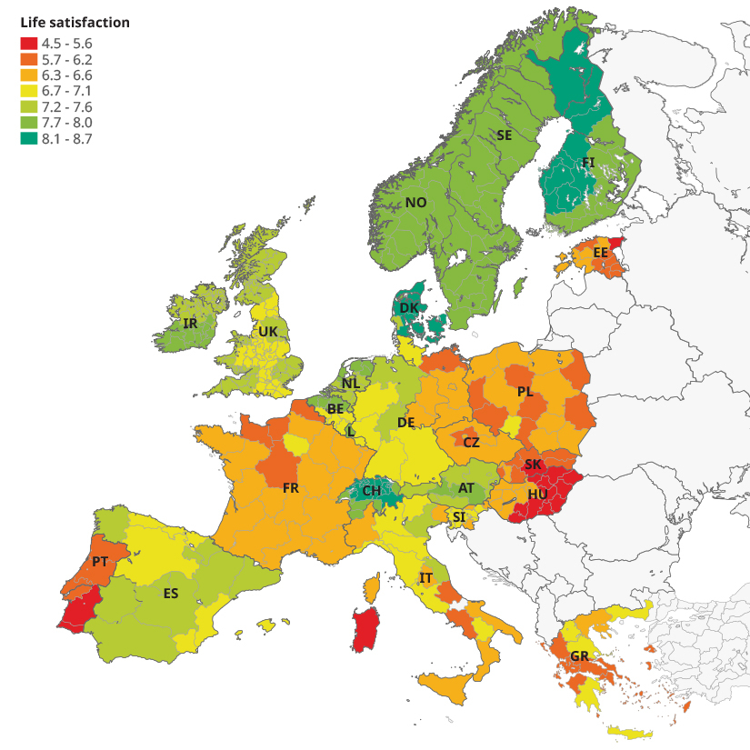
Figure 2: SO2 concentrations in Europe 2006
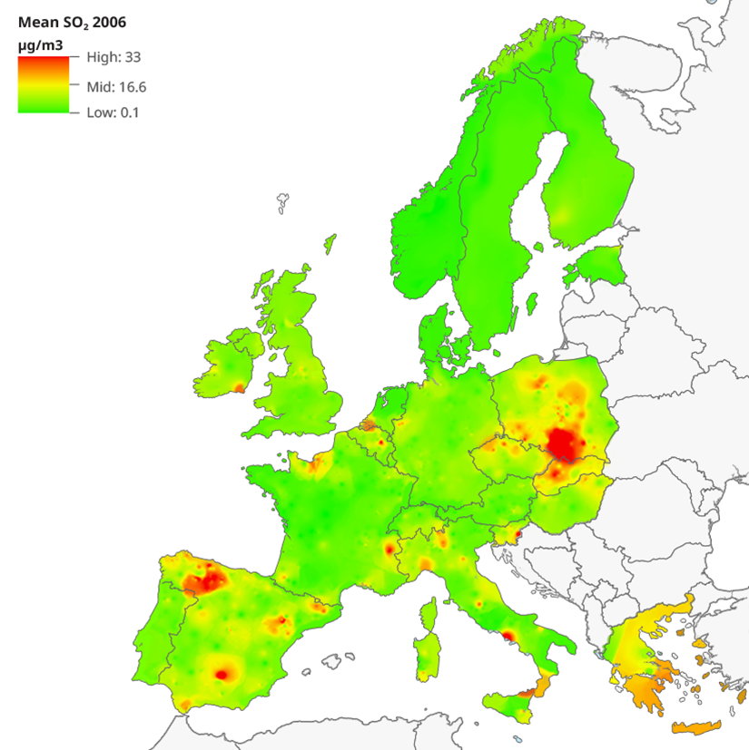
Figure 2 presents average SO2 concentrations at regional level across Europe in 2006. Similar to regional life satisfaction scores, for air pollution levels we also observe not only cross-national differences but also within-country variation. Thus, for example, Poland had an average SO2 concentration of 10.60 μg/m3 at national level but ranging between 4.8 μg/m3 and 21.22 μg/m3 across different regions.
If we compare Figures 1 and 2 we see that the countries with the lowest SO2 concentrations – Norway and Denmark – are also among the countries with the highest life satisfaction. Within countries such as Poland the areas where SO2 concentrations are highest (showing in red and orange in Figure 2) are also those areas where life satisfaction tends to be lower than average (showing in red and orange in Figure 1). There is a significant negative correlation (ρ=-0.125) between life satisfaction and SO2 levels at the regional level.
Statistical modelling was used to take account of the possibility that life satisfaction may also be influenced by a range of individual characteristics such as age, gender, income, self-reported health status, marital status and employment status as well as other regional level factors such as GDP and unemployment rates (see Appendix Table A.1 for details of the data used in this analysis). The results of this analysis confirm that the negative association between SO2 levels and life satisfaction is robust and remains apparent even after taking these other factors into account. An increase in SO2 concentrations by 1 μg/m3 is associated with a statistically significant reduction in life satisfaction of between 0.016 and 0.030 points on the 11-point life satisfaction scale. This is higher than previous estimates at national level, which range between 0.003 and 0.006 points for the same increase in SO2 concentrations (Ferreira et al. 2013). The analysis further suggests that SO2 has an indirect impact on life satisfaction through health, i.e. higher SO2 concentrations are associated with poorer health which in turn is associated with lower life satisfaction. However, much of negative impact of SO2 on life satisfaction is a direct effect not captured by physical health-related factors. This demonstrates the importance of studying the effect of environmental factors on people’s wider wellbeing.
Conclusion
Air quality and its effect on public health and welfare is an important concern for policymakers. The analysis presented here provides further evidence of the link between air pollution and individuals’ wellbeing, demonstrating a significant negative relationship between concentrations of SO2 in the atmosphere and life satisfaction across Europe. The particular contribution of this study, linking high quality survey data from the ESS with rich contextual data to carry out detailed regional level analysis across multiple European countries, has been to demonstrate that the association between pollution levels and wellbeing may be even stronger than previous analysis at national level has suggested. This finding confirms the important role that environmental factors may play in influencing subjective wellbeing and the need for policymakers to remain vigilant in monitoring air quality and enforcing standards.
The research discussed here was carried out as part of a collaborative research project ‘HAPPINESS’ (HAPpiness, Political Institutions, Natural Environment and Space), funded by the European Science Foundation and involving researchers from University College Dublin, Ireland; University of Gothenburg, Sweden; University of Navarra, Spain; University of Stirling, UK; and the University of Georgia, USA.
For more information on the merging of pollution and climate variables with the ESS in the HAPPINESS project, see:
Brereton, F., Moro, M., Ningal, T., Ferreira, S. (2011)
Technical report on GIS analysis, mapping and linking of contextual data to the European Social Survey. Dublin.
For full details of the analysis of SO2 levels and wellbeing presented here see:
Ferreira, S., Akay, A., Brereton, F., Cuñado, J., Martinsson, P., Moro, M., Ningal, T. (2013)
‘Life Satisfaction and Air Quality in Europe’. Ecological Economics, 88 (1), pp. 1-10.
Brereton, F., Moro, M., Ningal, T., Ferreira, S. (2011)
Technical report on GIS analysis, mapping and linking of contextual data to the European Social Survey. Dublin.
Ferreira, S., Akay, A., Brereton, F., Cuñado, J., Martinsson, P., Moro, M., Ningal, T. (2013)
‘Life Satisfaction and Air Quality in Europe’. Ecological Economics, 88 (1), pp. 1-10.
Ferrer-i-Carbonell, A. and Gowdy, J. (2007)
‘Environmental Degradation and Happiness’. Ecological Economics, 60, pp. 509-516.
Folinsbee, L.J. (1992)
‘Human Health Effects of Air Pollution’. Environmental Health Perspectives, 100, pp. 45–56.
Frey, B., Luechinger, S., Stutzer, A. (2009)
‘The Life Satisfaction Approach to Valuing Public Goods: The Case of Terrorism’. Public Choice, 138, pp. 317-345.
Rehdanz, K., Maddison, D. (2005)
‘Climate and Happiness’. Ecological Economics, 52, pp. 111-125.
Welsch, H. (2002)
‘Preferences over Prosperity and Pollution: Environmental Valuation Based on Happiness Surveys’. Kyklos, 55, pp. 473-494.
Welsch, H. (2006)
‘Environment and Happiness: Valuation of Air Pollution Using Life Satisfaction Data’. Ecological Economics, 58, pp. 801-813.
Van Praag, B., Baarsma, B. (2005)
‘Using Happiness Surveys to Value Intangibles: The Case of Airport Noise’. Economic Journal, 52, pp. 111-125.
Table A.1: ESS and contextual variables included in analysis
| Socio-demographic Indicators | ESS | |
|---|---|---|
| Subjective Wellbeing (“How satisfied with life as a whole?”) | 0 (extremely dissatisfied) – 10 (extremely satisfied) | |
| Sex | Dummy: 1= Female | |
| Age | Age of respondent in years | |
| Marital Status | 4 categories: married or in civil partnership; separated, divorced; widowed; never married nor in civil partnership (reference category) | |
| Household Income | Household’s total net income (all sources) | |
| Employment Status | 8 categories: paid work; in education; unemployed and actively looking for job; unemployed and not actively looking for job; permanently sick or disabled; retired; housework; other (reference category) | |
| Educational Level | Years of full-time education completed | |
| Household size | Number of people living regularly as member of household | |
| Children | Dummy: 1= Children in the household | |
| Citizenship | Dummy: 1=Citizen of country of residence | |
| Born in country | Dummy: 1=Born in country of residence | |
| Size of settlement | 5 categories: big city; suburbs; town/small city; village; farm/countryside (reference category) | |
| Personal and interpersonal feelings and functionings | ESS | |
| Health Status (self-reported) | Discrete: 1 (very good) – 5 (very bad) | |
| Religiosity | Dummy: 1 = Belonging to a particular religion or denomination | |
| Important to care for nature and environment | Discrete: 1 (very much like me) – 6 (not like me at all) | |
| Regional variables (up to NUTS3 level) | ||
| Pollution variables | EEA AirBase/Authors | |
| PM10 | PM10 mean annual concentration (μg/m3) | |
| CO | CO mean annual concentration (mg/m3) | |
| SO2 | SO2 mean annual concentration (μg/m3) | |
| NO | NO mean annual concentration (μg/m3) | |
| NO2 | NO2 mean annual concentration (μg/m3) | |
| Climate variables | ECA/Authors | |
| Mean annual temperature | Annual mean temperature (°C) | |
| July max temperature | Mean of daily max. temperature in July (°C) | |
| Jan min temperature | Mean of daily min. temperature in January (°C) | |
| Mean annual precipitation | Annual mean precipitation (mm) | |
| Socioeconomic structure | Eurostat/Authors | |
| GDP per capita | Regional gross domestic product (PPP per inhabitant) by NUTS 2 regions | |
| Population density | Population density by NUTS 2 region | |
| Unemployment rate | Unemployment rate by NUTS 2 region | |
Data source: Reproduced from Ferreira et al., 2013 (pp. 6-7).
- The HAPPINESS project, University College Dublin.
- The Nomenclature of Territorial Units (NUTS) is a regional classification developed for EU/EFTA countries for statistical purposes. Data may be available at one of 3 levels (NUTS1, NUTS2 or NUTS3) depending on the country, with NUTS 3 referring to the smallest geographical unit.
- Austria, Belgium, Czech Republic, Switzerland, Germany, Denmark, Estonia, Spain, Finland, France, Greece, Hungary, Ireland, Italy, Luxembourg, Netherlands, Norway, Poland, Portugal, Sweden, Slovenia, Slovakia and the UK. Ukraine was excluded due to difficulty obtaining some of the contextual data.
- Air Quality e-Reporting (AQ e-Reporting)
Similar to regional life satisfaction scores, for air pollution levels we also observe not only
cross-national differences but also within-country variation

Satisfied with democracy, satisfied with life?
Analysis of the European Social Survey (ESS) module on ‘Europeans’ Understandings and Evaluations of Democracy’ suggests that people are more satisfied with life in countries where the quality of democracy is high and when they believe in the legitimacy of their democratic regime.
Introduction
As early as Athenian times, Aristotle recognized that one of the main virtues of democracy is its capacity to lead a good life and happiness. Even nowadays, with many voices warning about a crisis of democracy in some European countries, most people around the world tend to think that democracy is still preferable to any other political regime and that people live better lives under democratic governments. Despite this optimistic vision, the question of whether democracy does indeed improve subjective wellbeing remains contested and there is evidence pointing in both directions. Some studies suggest that democracy vastly contributes to increasing people’s wellbeing (Owen, Videras and Willemsen, 2008; Orviska, Caplanova and Hudson, 2014); whereas for others, people’s wellbeing is mostly deemed to be independent of how democratic a country is (Stadelmann-Steffen and Vatter, 2012).
The question about the existence of a relationship between democratic performance and subjective wellbeing is not a trivial one. Certainly, democracy seems to be here to stay, and is generally perceived as a quasi-moral good. But, if democracy does not effectively contribute to increasing individual wellbeing, are we perhaps committing to an ill-fitted political regime? On the other hand, if there is a link between democratic performance and wellbeing, efforts to increase the quality of democracy may have a direct impact on citizens’ subjective wellbeing.
Using ESS data to explore the link between democracy and wellbeing
Thanks to Round 6 (2012/2013) of the European Social Survey (ESS) we are now in a better position to answer the question of whether there is a direct link between democracy and wellbeing, at least in the European context. Round 6 of the ESS includes a module on ‘Europeans’ Understandings and Evaluations of Democracy’, which provides for the first time a comprehensive measure of Europeans’ views and evaluations of democracy. These data allow for a more reliable test of the relationship between democratic performance and subjective wellbeing, both at the individual and the country level, than has previously been possible.
In the analysis that follows, which covers all 29 countries included in ESS Round 6,1 we use data from the democracy module and a question from the ESS core questionnaire which provides a measure of respondents’ self-assessed satisfaction with life (B20) to explore the link between satisfaction with democracy and satisfaction with life.
B20. All things considered, how satisfied are you with your life as a whole nowadays? Please answer using this card, where 0 means extremely dissatisfied and 10 means extremely satisfied.
Meet the author
Mónica Ferrín
Researcher, University of Zurich, Switzerland
| Extremely dissatisfied | Extremely satisfied | |||||||||
| 00 | 01 | 02 | 03 | 04 | 05 | 06 | 07 | 08 | 09 | 10 |
The ESS Round 6 module on ‘Europeans’ Understandings and Evaluations of Democracy’ aims to provide detailed data on citizens’ attitudes to democracy. To this end, the module focuses on two aspects of people’s attitudes to democracy:
- People’s beliefs and expectations as to how democracy should be. This was measured by asking respondents about the importance they attached to a list of democratic attributes on a scale from 0 ‘not at all important’ to 10 ‘extremely important’.
- People’s evaluations of how democracy performs in practice. Respondents were asked to rate the extent to which their country performs according to the same list of democratic attributes on a scale from 0 ‘Does not apply at all in country’ to 10 ‘Applies completely in country’.
The module assumes a multidimensional concept of democracy, which supported theoretically the choice of the list of attributes the respondents are asked about (see European Social Survey, 2013 for more details). Six different dimensions of democracy are identified: an electoral dimension, liberal dimension, social dimension, direct democracy dimension, inclusiveness dimension, and type of representation dimension.
Democratic performance and subjective wellbeing across European countries
At the country level, subjective wellbeing varies across countries in a similar way to democratic performance. Figure 1 confirms previous findings (Inglehart and Klingemann, 2000) and shows that in countries such as the Nordic countries, where democracy performs better (as measured by the World Bank’s Worldwide Governance Indicators (www.govindicators.org)), levels of satisfaction with life are higher than in countries where democracy performs worse (such as Russia or Ukraine). The correlation between average satisfaction with life and democratic performance is 0.79.
Figure 1: Correlation between life satisfaction and quality of democracy
Data source: ESS Round 6 (2012/2013) and Worldwide Governance Indicators (2012). Design weights applied to ESS data.
However, although it appears to support the hypothesis that democracy enhances wellbeing, Figure 1 may in fact depict a spurious relationship between democracy and life satisfaction. Since democratic performance goes hand in hand with economic performance, wellbeing might be related to economic wealth rather than to democratic quality. In addition, we find in Figure 1 countries with very different degrees of democratic quality displaying very similar levels of satisfaction with life (see, for example, Russia and Kosovo as compared to Lithuania and Portugal). In order to ascertain whether there is indeed a link between democratic quality and satisfaction with life, we also need to consider the relationship at the individual level i.e. do people who hold more positive views of their democracy also have higher wellbeing?
Democratic legitimacy and subjective wellbeing among Europeans
The study of citizens’ attitudes to democracy is framed by the concept of democratic support (Easton, 1965; Easton, 1975). Underlying this concept is the idea that a democracy persists (and ultimately performs well), only when it is supported by its citizens. Using Round 6 (2012/2013) of the ESS, we are able to measure one of the main components of democratic support: Europeans’ beliefs of democratic legitimacy – or the evaluation of democratic performance in the light of some set of ideal standards. The higher the congruence between democratic evaluations (what democracy is) and democratic ideals (how democracy should be), the more strongly an individual believes their democratic regime is legitimate.
This concept of democratic legitimacy fits particularly well with the arguments developed in the literature regarding the relationship between democracy and wellbeing. Subjective wellbeing (or the utility an individual derives from something) is composed both of emotions provoked by different aspects of life (how important they are considered to be), and individuals’ judgments regarding how far these same aspects are realised either in absolute terms or relative to other people (Frey and Stutzer, 2002). As related to politics, the argument is that the more policy outcomes match with an individual’s preferences, the higher their levels of subjective wellbeing will be (Stadelmann-Steffen and Vatter, 2012; Tavits, 2008). It has previously been argued that, in a well-functioning democratic system, politicians are more responsive to citizens’ preferences – and less corrupt – so subjective wellbeing should be higher (Orviska, Caplanova and Hudson, 2014; Tay, Herian and Diener, 2014). Using the ESS we can now test directly whether there is an effect of democracy on wellbeing. Is greater perceived legitimacy i.e. greater congruence between citizens’ ideals and evaluations of democracy associated with higher life satisfaction?
Considering that democracy is a multidimensional concept, in the analysis that follows we distinguish between: liberal democracy legitimacy beliefs (i.e. beliefs concerning democratic procedures ); social democracy legitimacy beliefs (beliefs concerning social outcomes); and direct democracy legitimacy beliefs (focusing on participatory mechanisms) (see Appendix for details of how these measures have been constructed). This distinction is driven by an analysis of Europeans’ views of democracy, which appear to be ordered within these three democratic dimensions (Kriesi, Willem and Moncagatte, forthcoming). The specific construction of the three legitimacy scales is based on the approach described by Wessels (forthcoming). From the point of view of subjective wellbeing, it is relevant to consider which of these three types of legitimacy – if any – has a stronger impact on citizens’ utility function.
Figure 2 summarises the results of multilevel regression analysis to uncover the relative importance of a range of different individual and country level factors in predicting satisfaction with life (see Appendix Table A.1 for full results). Corresponding with previous findings, female, married, religious, wealthier and healthier people tend to be more satisfied with life than others. Most interesting for this study is the association between legitimacy beliefs and satisfaction with life. We find a significant positive association between each of the three measures of legitimacy and satisfaction with life. This is the case even after controlling for individual characteristics and the economic performance of the country, supporting the idea that it is not only economics which matters for satisfaction.2 The more a system is perceived as legitimate (that is, the more a democracy is perceived as performing according to an individual’s ideals), the higher is subjective wellbeing. It is notable that beliefs about the legitimacy of democratic social outcomes are more strongly associated with satisfaction than attitudes towards democratic procedures or the availability of mechanisms for direct participation. Democracy is important for wellbeing but some aspects of democratic performance appear to matter more than others.
Figure 2: Predictors of life satisfaction
Data source: ESS Round 6 (2012/2013).
Note: Selected coefficients from multilevel regression analysis and corresponding 95% confidence intervals. Dots to the right (left) of the vertical red line indicate a significant positive (negative) association with life satisfaction. Age and education not significantly associated with life satisfaction.
Comparing more and less democratic countries
But, does this positive relationship between democracy and wellbeing hold in all contexts? Previous studies have found that the relationship between democratic performance and wellbeing differs depending on the economic wealth of a country (Veenhoven, 2000).3 We might also expect the quality of democracy, measured objectively, to condition how much perceived democratic legitimacy matters for individuals’ satisfaction with life; the relative importance attached to expectations and the failure of reality to live up to these expectations may vary under different levels of democratic performance.
Figure 3 shows the strength of the relationship between life satisfaction and perceived democratic legitimacy (for each of the liberal, social and direct democracy dimensions) for countries judged as being of low, medium and high democratic quality according to the Worldwide Governance Indicators (see Appendix Table A.2 for full details of this analysis). The lines in the bottom third of Figure 3 show the relationship between legitimacy beliefs and wellbeing in low quality democracies and the lines in the top third of Figure 3 show the relationship in high quality democracies. Interestingly, the effect of democratic legitimacy beliefs on life satisfaction is stronger the less the objective democratic quality of a country. In countries where democracy performs worst (as measured by Worldwide Governance Indicators), beliefs that the system is nevertheless legitimate clearly make citizens more satisfied with their lives, whereas in countries where democratic performance is better there is a much weaker relationship between legitimacy beliefs and wellbeing. It may be that, in high quality democracies, citizens have become used to the good functioning of democracy and, therefore, their subjective perceptions as to whether democracy is or is not performing quite as well as they would like play a less significant role in their satisfaction with life.
Figure 3: Effect of legitimacy beliefs on life satisfaction by quality of democracy
Data source: ESS Round 6 (2012/2013).
Note: Marginal effect of legitimacy beliefs on satisfaction with life (0-10) based on results of multilevel regression.
Conclusion
The analysis presented here suggests that the general optimism about the virtue of democracy is not without grounds. Countries where the quality of democracy is high also tend to have citizens who are more satisfied in general with their lives. Making use of a unique battery of questions exploring individuals’ attitudes to democracy fielded as part of the ESS Round 6 (2012/2013), we have also shown that, within countries, individuals are more satisfied with their own lives if they perceive their democracy to be legitimate i.e. if they believe that democracy in their country is performing according to how they think democracy should be. This finding highlights the importance of democratic legitimacy not only in ensuring the continuation of democratic regimes but also for ensuring the wellbeing of the population. The challenge for governments across Europe, especially but not only those in low quality democracies, is to do everything they can to improve democratic performance in line with citizens’ expectations.
To find out more about the ESS module on ‘Europeans’ Understandings and Evaluations of Democracy’ and to read findings based on these data please see the following resources:
European Social Survey (2013)
Round 6 Module on Europeans’ Understandings and Evaluations of Democracy – Final Module in Template. London: Centre for Comparative Social Surveys.
Ferrin, M., Kriesi, H.-P., Morlino, M., Magalhaes, P., Alonso, S., Wessels, B. (2014)
Europeans’ Understandings and Evaluations of Democracy: Topline Results from Round 6 of the European Social Survey. London: Centre for Comparative Social Surveys.
Ferrín, M. and Kriesi, H. (ed) (forthcoming)
How Europeans View and Evaluate Democracy. Oxford: Oxford University Press.
Bryk, A.S. and Raudenbush, S.W. (1992)
Hierarchical Linear Models. Newbury Park, Sage.
Easton, D. (1965)
A Systems Analysis of Political Life. New Jersey: Wiley.
Easton, D. (1975)
‘A Re-assessment of the Concept of Political Support’. British Journal of Political Science, 5(4), pp. 435–457.
European Social Survey (2013)
Round 6 Module on Europeans’ Understandings and Evaluations of Democracy – Final Module in Template. London: Centre for Comparative Social Surveys.
Ferrin, M., Kriesi, H.-P., Morlino, M., Magalhaes, P., Alonso, S., Wessels, B. (2014)
Europeans’ Understandings and Evaluations of Democracy: Topline Results from Round 6 of the European Social Survey. London: Centre for Comparative Social Surveys.
Frey, B. S. and Stutzer, A. (2002)
‘What Can Economists Learn from Happiness Research? ’ Journal of Economic Literature, 40(2), pp. 402–435.
Inglehart, R. and Klingemann, H. (2000)
‘Genes, Culture, Democracy, and Happiness’. In: Diener, E. and Suh, E.M. (ed) Culture and Subjective Well-being. Cambridge: MIT Press, pp. 165–183.
Kriesi, H., Willem, S., Moncagatte, P. (forthcoming)
‘The Structure of Europeans’ Views of Democracy: Citizens’ Models of Democracy’. In: Ferrín, M. and Kriesi, H. (ed) How Europeans View and Evaluate Democracy. Oxford: Oxford University Press.
Orviska, M., Caplanova, A., Hudson, J. (2014)
‘The Impact of Democracy on Well-Being’. Social Indicators Research, 115(1), pp. 493–508.
Owen, A. L., Videras, J. and Christina Willemsen (2008)
‘Democracy, Participation, and Life Satisfaction’. Social Science Quarterly, 89(4), pp. 987–1005.
Stadelmann-Steffen, I. and Vatter, A. (2012)
‘Does Satisfaction with Democracy Really Increase Happiness? Direct Democracy and Individual Satisfaction in Switzerland’. Political Behavior, 34(3), pp. 535–559.
Tavits, M. (2008)
‘Representation, Corruption, and Subjective Well-Being’. Comparative Political Studies, 41(12), pp. 1607–1630.
Tay, L., Herian, M.N. and Diener, E. (2014)
‘Detrimental Effects of Corruption and Subjective Well-Being Whether, How, and When’. Social Psychological and Personality Science, 5(7), pp. 751–759.
Veenhoven, R. (2000)
‘Freedom and Happiness: A Comparative Study in Forty-four Nations in the Early 1990s’. In: Diener, E. and Suh, E.M. (ed) Culture and Subjective Well-being. Cambridge: MIT Press, pp. 257–288.
Wessels, B. (forthcoming)
‘Democratic Legitimacy: Concepts, Measures, Outcomes’. In: Ferrín, M. and Kriesi, H. (ed) How Europeans View and Evaluate Democracy. Oxford: Oxford University Press.
Construction of ‘beliefs about democratic legitimacy’ scales
Perceived democratic legitimacy is defined as the balanced distance between an individual’s (i) views regarding their ideal democracy and their evaluations of their actual democracy. Individuals’ perceptions of a number of different aspects of democracy (j) are combined to create an overall score for each of the three dimensions of democracy identified: liberal, social and direct democracy.
Perceived legitimacyi = Σ(evaluationij-viewij)*viewij
The resulting value is rescaled to be between 0-1 and where evaluation > view this is replaced by the value 1 in the calculation. See Wessels (forthcoming) for more information on the operationalization of this measure.
In Round 6 (2012/2013) of the ESS respondents’ views and evaluations of democracy are measured as follows:
View
E1. Using this card, please tell me how important you think it is for democracy in general... that national elections are free and fair.
| Not at all important for democracy in general | Extremely important | |||||||||
| 00 | 01 | 02 | 03 | 04 | 05 | 06 | 07 | 08 | 09 | 10 |
Evaluation
E17. Using this card, please tell me to what extent you think each of the following statements applies in [country]. National elections in [country] are free and fair.
| Does not apply at all | Applies | |||||||||
| 00 | 01 | 02 | 03 | 04 | 05 | 06 | 07 | 08 | 09 | 10 |
The different aspects of democracy about which respondents were asked and which make up each dimension are shown below. The three legitimacy scales are based on an empirical classification of respondents’ views of democracy. According to Kriesi, Willem and Moncagatte (forthcoming), Europeans’ views of democracy are hierarchically ordered along these three dimensions: the liberal, the social, and the direct democracy dimensions.
Liberal democracy legitimacy beliefs
- National elections are free and fair
- Voters discuss politics with people they know before deciding how to vote
- Different political parties offer clear alternatives to one another
- Opposition parties are free to criticise the government
- The media are free to criticise the government
- The media provide citizens with reliable information to judge the government
- The rights of minority groups are protected
- The courts treat everyone the same
- Governing parties are punished in elections when they have done a bad job
- Government explains its decisions to voters
- Politicians take into account the views of other European governments before making decisions
Social democracy legitimacy beliefs
- The government takes measures to reduce differences in income levels
- The government protects all citizens against poverty
Direct democracy legitimacy beliefs
- Citizens have the final say on the most important political issues by voting on them directly in referendums
Modelling satisfaction with life as a function of democratic legitimacy
Hierarchical linear modelling (HLM) was used to analyse the relationship between life satisfaction and emotional experience. HLM takes account of the fact that ESS data are hierarchically ordered with individuals (the Level 1 units of analysis) nested within countries (the Level 2 units of analysis) and the possibility that parameters which vary across individuals may also vary across countries depending on country-level characteristics (see Bryk and Raudenbush, 1992). It provides the means to estimate the amount of variance in the dependent variable (in this case life satisfaction, 0-10) explained by both individual and country level factors taking into account the likely inter-correlation between individuals nested within the same country.
Table A.1: Relationship between life satisfaction (0-10) and perceived democratic legitimacy: Results from hierarchical linear modelling
| Dependent variable | |
|---|---|
| INDEPENDENT VARIABLES | LIFE SATISFACTION |
| Age | 0.012*** |
| (-0.001) | |
| Male (1) | -0.156*** |
| (-0.021) | |
| Level of education (1-4) | 0.001 |
| (-0.012) | |
| Civil status: Divorced (ref. married) | -0.477*** |
| (-0.034) | |
| Civil status: Widowed (ref. married) | -0.220*** |
| (-0.039) | |
| Civil status: Single (ref. married) | -0.144*** |
| (-0.033) | |
| Has children (1) | -0.165*** |
| (-0.030) | |
| Is employed (1) | -0.061*** |
| (-0.024) | |
| Income (1= 1st decile – 10= 10th decile) | 0.124*** |
| (-0.004) | |
| Is religious | 0.143*** |
| (-0.023) | |
| How healthy (1=very bad health – 5= very good health) | 0.664*** |
| (-0.013) | |
| Liberal democracy legitimacy | 0.113*** |
| (-0.017) | |
| Social democracy legitimacy | 0.199*** |
| (-0.015) | |
| Direct democracy legitimacy | 0.045*** |
| (-0.013) | |
| Change in growth rates 2005/2008 – 2009/2012 | 0.172*** |
| (-0.060) | |
| Constant | 4.020*** |
| (-0.277) | |
| Observations | 41,304 |
| Number of groups | 29 |
| Variance components | |
| sd(country) | 0.654 |
| sd(individual) | 2.002 |
Data source: European Social Survey Round 6 (2012/2013). World Bank (2005-2012) for growth rates.
Note: * p < 0.05; ** p < 0.01; *** p < 0.001. Standard errors in parentheses.
Table A.2: Relationship between life satisfaction (0-10) and perceived democratic legitimacy including interaction between perceived democratic legitimacy and objective democratic quality: Results from hierarchical linear modelling
| Dependent Variable | |||
|---|---|---|---|
| INDEPENDENT VARIABLES | LIFE SATISFACTION | ||
| Age | 0.012*** | 0.012*** | 0.012*** |
| (-0.001) | (-0.001) | (-0.001) | |
| Male (1) | -0.153*** | -0.150*** | -0.154*** |
| (-0.021) | (-0.021) | (-0.021) | |
| Level of education (1-4) | -0.001 | 0.001 | 0.000 |
| (-0.012) | (-0.012) | (-0.012) | |
| Civil status: Divorced (ref. married) | -0.480*** | -0.481*** | -0.479*** |
| (-0.034) | (-0.034) | (-0.034) | |
| Civil status: Widowed (ref. married) | -0.220*** | -0.216*** | -0.221*** |
| (-0.039) | (-0.039) | (-0.039) | |
| Civil status: Single (ref. married) | -0.147*** | -0.147*** | -0.146*** |
| (-0.033) | (-0.033) | (-0.033) | |
| Has children (1) | -0.166*** | -0.167*** | -0.166*** |
| (-0.030) | (-0.030) | (-0.030) | |
| Is employed (1) | -0.061*** | -0.063*** | -0.062*** |
| (-0.024) | (-0.024) | (-0.024) | |
| Income (1= 1st decile – 10= 10th decile) | 0.124*** | 0.124*** | 0.124*** |
| (-0.004) | (-0.004) | (-0.004) | |
| Is religious | 0.149*** | 0.152*** | 0.148*** |
| (-0.023) | (-0.023) | (-0.023) | |
| How healthy (1=very bad health – 5= very good health) | 0.665*** | 0.665*** | 0.665*** |
| (-0.013) | (-0.013) | (-0.013) | |
| Liberal democracy legitimacy | 0.823*** | 0.570*** | 0.586*** |
| (-0.109) | (-0.093) | (-0.093) | |
| Social democracy legitimacy | 0.616*** | 0.839*** | 0.606*** |
| (-0.046) | (-0.063) | (-0.046) | |
| Direct democracy legitimacy | 0.144*** | 0.143*** | 0.269*** |
| (-0.041) | (-0.041) | (-0.059) | |
| Democratic quality: Medium (ref. low quality) | 0.733*** | 0.599*** | 0.586** |
| (-0.246) | (-0.226) | (-0.229) | |
| Democratic quality: High (ref. low quality) | 1.698*** | 1.514*** | 1.370*** |
| (-0.282) | (-0.246) | (-0.249) | |
| Interaction: Medium quality#liberal legitimacy scale | -0.338** | ||
| (-0.144) | |||
| Interaction: High quality#liberal legitimacy scale | -0.685*** | ||
| (-0.185) | |||
| Interaction: Medium quality#social legitimacy scale | -0.234*** | ||
| (-0.080) | |||
| Interaction: High quality#social legitimacy scale | -0.575*** | ||
| (-0.089) | |||
| Interaction: Medium quality#direct legitimacy scale | -0.144* | ||
| (-0.075) | |||
| Interaction: High quality#direct legitimacy scale | -0.291*** | ||
| (-0.086) | |||
| Change in growth rates 2005/2008 – 2009/2012 | 0.094** | 0.094** | 0.092* |
| (-0.047) | (-0.047) | (-0.048) | |
| Constant | 2.119*** | 2.193*** | 2.201*** |
| (-0.294) | (-0.291) | (-0.293) | |
| Observations | 41,304 | 41,304 | 41,304 |
| Number of groups | 29 | 29 | 29 |
| Variance components | |||
| sd(country) | 0.483 | 0.482 | 0.485 |
| sd(individual) | 2.001 | 2.001 | 2.001 |
Data source: European Social Survey Round 6 (2012/2013). World Bank (2005-2012) for growth rates and Worldwide Governance Indicators (2012) for measure of democratic quality.
Note: * p < 0.05; ** p < 0.01; *** p < 0.001. Standard errors in parentheses.
To test the interaction between perceived democratic legitimacy and objective democratic quality the sample was divided in three groups of similar size, cross-checked by theoretical consistency, based on countries’ score on the summary index of the Worldwide Governance Indicators. Group 1 = low democratic quality (Albania, Bulgaria, Hungary, Israel, Italy, Lithuania, Russia, Slovakia, Ukraine, Kosovo). Group 2 = medium democratic quality (Belgium, Cyprus, Czech Republic, Estonia, France, UK, Poland, Portugal, Slovenia, Spain). Group3 = high democratic quality (Denmark, Finland, Germany, Ireland, Iceland, Netherlands, Norway, Sweden, Switzerland).
- A total sample of around 54,600 respondents.
- Economic growth is measured in terms of the change in average GDP growth 2005-2008 to 2009-2012. Source: World Development Indicators
- Veenhoven (2000) finds that freedom (conceived as a chance to choose) is positively related to happiness in rich countries; but the same relationship does not hold in poor countries.
Can we be satisfied with life without being happy? Life satisfaction and emotional experience
In general people who experience more positive emotions also feel more satisfied with life. However, analysis of the European Social Survey (ESS) suggests that the importance of positive emotions varies across countries depending on cultural values.
Introduction
At first glance, it appears self‐evident that positive emotions enhance our life satisfaction, whereas negative emotions bring us down and decrease our satisfaction with life. However, the question remains as to whether we can be satisfied with life without being happy? Moreover, are there cultural differences in the relationships among life satisfaction, positive emotions, and negative emotions? And, if there are, how can these differences be explained? These are the main questions we seek to answer using data from 29 countries which participated in Round 6 (2012/2013) of the European Social Survey (ESS).
Subjective wellbeing and its components
Life satisfaction, positive and negative emotions can be considered the main components of subjective wellbeing defined as “a person’s cognitive and affective evaluations of his or her life“ (Diener, Lucas and Oishi, 2002: p. 63). The judgment of how satisfied people are with their life is based on a comparison with a standard that each individual sets for themselves (Diener et al., 1985). However, subjective wellbeing also has an affective side, which depends on the experience of different emotions, positive as well as negative. The affective component of subjective wellbeing depends primarily on the frequency and not on the intensity of affective experiences (Diener et al., 1991).
There is evidence that people from different cultures assess positive or negative emotions differently in determining how satisfied they are with their lives (Kuppens, Realo and Diener, 2008) and that the strength of the relationship between life satisfaction and affective components of subjective wellbeing depends on many different factors, such as cultural values (Kuppens, Realo and Diener, 2008; Suh et al., 1998) and personality traits (Kööts-Ausmees, Realo and Allik, 2013), among others.
Exploring subjective wellbeing using the ESS
Here we examine how the experience of positive and negative emotions is related to life satisfaction across 29 European nations, using data from Round 6 of the ESS collected in 2012/2013.1 The ESS is a valuable source of data with which to explore this relationship for two reasons. First, it provides comparable data for nationally representative samples collected to the highest methodological standards across countries. Second, it includes a range of different indicators of subjective wellbeing including measures of life satisfaction and data about the frequency of emotional experience in the last week.
As part of the ESS core questionnaire, respondents were asked to rate how satisfied they were with their life as a whole on a 0-10 scale:
B20. All things considered, how satisfied are you with your life as a whole nowadays? Please answer using this card, where 0 means extremely dissatisfied and 10 means extremely satisfied.
| Extremely dissatisfied | Extremely satisfied | |||||||||
| 00 | 01 | 02 | 03 | 04 | 05 | 06 | 07 | 08 | 09 | 10 |
As part of the rotating module on ‘Personal and Social Wellbeing’ fielded in ESS Round 6 (2012/2013) respondents were also asked about their experience of positive and negative emotions. The frequency of four positive and four negative emotions2 during the past week was rated on a 1-4 scale, where 1 indicated very low occurrence (“none or almost none of the time”) and 4 indicated very high occurrence (“all or almost all of the time”).
D8 “How much of the time during the past week you were happy?”
D10 “How much of the time during the past week you enjoyed life?”
D13 “How much of the time during the past week you had a lot of energy?”
D15 “How much of the time during the past week you felt calm and peaceful?”
In the scale of Negative Affect we also included four items:
D5 “How much of the time during the past week you felt depressed?”
D9 “How much of the time during the past week you felt lonely?”
D11 “How much of the time during the past week you felt sad?”
D14 “How much of the time during the past week you felt anxious?”
1 = “none or almost none of the time”, 2 = “some of the time”, 3 = “most of the time”, 4 = “all or almost all of the time”
To the extent that the relationship among the components of subjective wellbeing is found to vary across different European countries, we are interested in exploring whether this might be explained by differences in cultural values. We focus here on the survival/self-expression cultural value dimension. This reflects the extent of the shift within societies from an emphasis on existential economic and physical security to the appreciation of individual autonomy, self-expression, and quality of life (Inglehart and Baker, 2000). Based on earlier research (Kuppens, Realo and Diener, 2008; Kööts-Ausmees, Realo and Allik, 2013) we expect that this value dimension will influence how European nations differ in weighing the affective building blocks of what constitutes a good life.
Survival versus self-expression is one of two dimensions of cross-cultural variation (the other being traditional versus secular-rational values) which emerged from analyses of the World Values Survey (WVS) data, the largest study of values, attitudes, and beliefs around the world (Inglehart and Welzel, 2005; Inglehart and Baker, 2000). Since 1981, six waves of surveys have been carried out in almost 100 countries containing almost 90 percent of the world’s population (http://worldvaluessurvey.org/). The above-mentioned two dimensions make it possible to chart each society that has participated in the WVS on a so-called ‘global map of cross-cultural variation’.
Broadly speaking, the survival/self-expression dimension reflects the shift from an emphasis on existential economic and physical security to the appreciation of individual autonomy, self-expression, and quality of life. According to Inglehart and Welzel (2005), the self-expression pole of the dimension “taps a syndrome of tolerance, trust, emphasis on subjective well-being, civic activism, and self-expression that emerges in post-industrial societies with high level of existential security and individual autonomy” (p. 52). At the opposite pole of the dimension, people in societies that emphasize survival values give priority to physical and economic security, tend to mistrust others, and value material possessions and income. As societies develop socially and economically, people’s values shift from survival values toward self-expression values. Higher scores on the dimension reflect higher levels of self-expression and lower scores reflect higher levels of survival.
In our analysis we use national mean scores of survival/self-expression based on country-level data from Wave 4 (2000) and Wave 5 (2005) of the World Values Survey (WVS).3 The scores were retrieved from the WVS website (www.worldvaluessurvey.org). Across the ESS Round 6 countries, self-expression was most highly valued in Sweden, whereas survival was most highly valued in Russia (see Appendix Table A.1).
Meet the authors
Anu Realo
Academy Research Professor, University of Tartu, Estonia
Liisi Kööts-Ausmees
Research Fellow of Personality Psychology, Department of Psychology, University of Tartu, Estonia
Jüri Allik
Professor of Experimental Psychology, Department of Psychology, University of Tartu, Estonia
Findings
To assess whether the relationship between life satisfaction and emotional experience is different across 29 European countries and whether the country-level value dimension of survival/self-expression moderates these differences, we conducted a series of multilevel linear modelling analyses to analyse the attitudes of individuals grouped within countries.
As predicted we find that, at the level of individuals, positive emotions are positively associated with life satisfaction, whereas negative emotions are negatively associated with life satisfaction (see Appendix Table A.2, Model 1). As in earlier studies (Kuppens, Realo and Diener, 2008; Kööts-Ausmees, Realo and Allik, 2013; Bastian et al., 2014), positive emotions predict life satisfaction judgments slightly more strongly than negative emotions. Note though that, although our findings clearly show that life satisfaction and emotional experiences are significantly related to each other, we need to be careful about inferring a causal relationship; on the basis of this evidence we cannot know whether the frequency of positive emotions influences life satisfaction judgments or vice versa.
Figures 1 and 2 provide support for our expectation that the contribution of positive and negative emotions to life satisfaction varies significantly across countries.
The
contribution
of positive and negative emotions to life satisfaction
varies significantly across countries
Figure 1: Strength of the relationship between life satisfaction and positive affect across 29 European countries
Data source: ESS Round 6 (2012/2013). Post-stratification weights applied.
Note: Life satisfaction was predicted by positive affect and negative affect scales in each of the 29 European countries in a series of multiple regression analyses.
Figure 2: Strength of the relationship between life satisfaction and negative affect across 29 European countries
Data source: ESS Round 6 (2012/13). Post-stratification weights applied.
Note: Life satisfaction was predicted by positive affect and negative affect scales in each of the 29 European countries in a series of multiple regression analyses.
The role of cultural values
We next examine the relationship between life satisfaction and emotional experiences in the context of country-level cultural values in order to test whether differences in the strength of this relationship between countries may be explained by differences in the extent to which survival versus self–expression is valued. Figure 3 shows how the importance attached to self-expression vs. survival varies across countries. The distribution of cultural values across countries can be compared with the varying strength of the relationship between emotions and life satisfaction as displayed in Figures 1 and 2 above (see also Appendix Table A.1). Statistical modelling shows that, in fact, only the relationship between positive emotions and life satisfaction judgments (and not negative emotions and life satisfaction judgements) is moderated by survival/self-expression values: countries that score higher on survival values generally seem to promote life satisfaction by emphasizing the importance of pleasant experiences (see Appendix Table A.3, Model 2).4 In sum, people in countries that emphasize survival values seem to need more positive emotions to be satisfied with their life than people in countries that rank high on self-expression. Lack of negative emotions, however, seems to be an equally necessary prerequisite for being satisfied with your life regardless of whether countries score high or low on survival/self-expression dimension.
People in countries that emphasize survival values seem to
need more positive emotions
to be satisfied with life
Figure 3: Survival versus self-expression values across 29 European countries
Data source: World Values Survey Wave 4 (2000) and Wave 5 (2006).
The role of socio-economic development
Given that countries that emphasize self-expression values tend to have higher levels of socio-economic development (Inglehart and Welzel, 2005), one might ask whether it is socio-economic development (and not survival/self-expression values) which moderates the relationship between life satisfaction and positive emotions. Additional analyses using the Human Development Index (HDI) as an indicator of countries’ level of socio-economic development shows that the relationship between life satisfaction and positive affect is indeed significantly weaker in countries with a high level of development (see Appendix Table A.3, Model 3).
It is, however, not possible to disentangle the effects of survival/self-expression and human development on the relationship between life satisfaction and positive emotions across the 29 European countries because the two country-level indicators are so highly correlated with one another.5 The stronger relationship between positive emotions and life satisfaction in some European countries may be explained either by a greater emphasis on survival over self-expression values in those countries and/or by a higher score on the HDI.
Conclusion
So, can we be satisfied with life without being happy? Our results show that in general, people appear to need positive emotions to feel satisfied with life but the maximization of pleasure and happiness is not equally important in all European countries. Rather it varies along with cultural values and the country’s level of development; people in survival-oriented countries and/or with a lower level of socioeconomic and human development appear to need more positive stimulation and emotions to be satisfied with life (see also Kööts-Ausmees, Realo and Allik, 2013).6
How could these findings be interpreted? In survival-oriented countries, where the level of human development is not very high and where people strive for security, life satisfaction is more strongly related to experiencing frequent positive emotions. On the other hand, in highly developed countries where self-expression is often also valued, the overall level of wellbeing of most individuals is already rather high and/or provided in other ways, so that they can be quite satisfied with life even when experiencing fewer pleasant emotions.
Our findings show how emotional aspects of the good life vary across European countries and that this depends at least partly on the values that characterize one’s culture. Although positive emotions might be universally viewed as desirable, there seem to be distinct cultural differences in how relevant such emotional experiences are to life satisfaction. Our findings help to understand that positive emotions matter and they are not just the opposite side of negative emotions. A happy and peaceful person is more likely to think that his or her life is great. However, these positive feelings seem to play a more crucial role in judging one’s life satisfaction in some societies – most notably in those where survival is uncertain – than in others.
To read more about the relationship between life satisfaction and emotional experiences across Europe see:
Kuppens, P., Realo, A., Diener, E. (2008)
‘The role of positive and negative emotions in life satisfaction judgment across nations’. Journal of Personality and Social Psychology, 95, pp. 66-75.
Kööts-Ausmees, L., Realo, A., Allik, J. (2013)
‘The relationship between life satisfaction and emotional experience in 21 European countries’. Journal of Cross-Cultural Psychology, 44, pp. 223-244.
Realo, A. and Dobewall, H. (2011)
‘Does life satisfaction change with age? A comparison of Estonia, Finland, Latvia, and Sweden’. Journal of Research in Personality, 45, pp. 297-308.
Anu Realo was a Fellow-in-Residence at the Netherlands Institute for Advanced Study (NIAS) while writing this article.
Bastian, B., Kuppens, P., De Roover, K., Diener, E. (2014)
‘Is valuing positive emotion associated with life satisfaction?’ Emotion, 14, pp. 639-645.
Bryk, A.S. and Raudenbush, S.W. (1992)
Hierarchical Linear Models. Newbury Park: Sage.
Diener, E., Colvin, C.R., Pavor, W.G., Allman, A. (1991)
‘The psychic costs of intense positive affect’. Journal of Personality and Social Psychology, 61, pp. 492-503
Diener, E., Emmons, R.A., Larsen, R.J., Griffin, S. (1985)
‘The satisfaction with life scale’. Journal of Personality Assessment, 49, pp. 71-75.
Diener, E., Lucas, R.E., Oishi, S. (2002)
‘Subjective well-being: The science of happiness and life satisfaction’. In: Snyder, C.R. and Lopez, S.J. (ed) Handbook of Positive psychology. Oxford: Oxford University Press, pp. 63-73.
Hofstede, G. (2001)
Culture’s Consequences: Comparing Values, Behaviors, Institutions and Organizations Across Nations. Beverly Hills: Sage.
Inglehart, R. and Baker, W.E. (2000)
‘Modernization, cultural change, and the persistence of traditional values’. American Sociological Review, 65, pp. 19-51.
Inglehart, R. and Welzel, C. (2005)
Modernization, Cultural Change, and Democracy: The Human Development Sequence. New York, NY: Cambridge University Press.
Kuppens, P., Realo, A., Diener, E. (2008)
‘The role of positive and negative emotions in life satisfaction judgment across nations’. Journal of Personality and Social Psychology, 95, pp. 66-75.
Kööts-Ausmees, L., Realo, A., Allik, J. (2013)
‘The relationship between life satisfaction and emotional experience in 21 European countries’. Journal of Cross-Cultural Psychology, 44, pp. 223-244.
Suh, E., Diener, E., Oishi, S. and Triandis, H.C. (1998)
‘The shifting basis of life satisfaction judgments across cultures: Emotions versus norms’. Journal of Personality and Social Psychology, 74, pp. 482-493
Tay, L. And Diener, E. (2011)
’Needs and subjective well-being around the world’. Journal of Personality and Social Psychology, 101, pp. 354-365.
Table A.1: Mean life satisfaction, survival/self-expression value scores, and the relationship between life satisfaction and emotional experience by country
| The relationship between life satisfaction and emotional experience (1) | ||||
|---|---|---|---|---|
| Country | Mean life satisfaction (s.d.) (1) | Survival/self-expression score (2) | Positive affect beta | Negative affect beta |
| Sweden | 7.87 | 2.35 | 0.37 | -0.19 |
| (-1.69) | ||||
| Norway | 8.12 | 2.17 | 0.27 | -0.39 |
| (-1.61) | ||||
| Switzerland | 8.17 | 1.9 | 0.27 | -0.3 |
| (-1.67) | ||||
| Denmark | 8.54 | 1.87 | 0.35 | -0.17 |
| (-1.54) | ||||
| UK | 7.36 | 1.68 | 0.36 | -0.18 |
| (-2.03) | ||||
| Iceland | 7.96 | 1.63 | 0.3 | -0.35 |
| (-1.63) | ||||
| Netherlands | 7.94 | 1.39 | 0.35 | -0.24 |
| (-1.48) | ||||
| Ireland | 6.82 | 1.18 | 0.29 | -0.21 |
| (-2.23) | ||||
| Belgium | 7.45 | 1.13 | 0.29 | -0.25 |
| (-1.75) | ||||
| France | 6.56 | 1.13 | 0.24 | -0.24 |
| (-2.43) | ||||
| Finland | 8.09 | 1.12 | 0.36 | -0.22 |
| (-1.41) | ||||
| Germany | 7.6 | 0.74 | 0.28 | -0.2 |
| (-2.03) | ||||
| Italy | 6.56 | 0.6 | 0.26 | -0.27 |
| (-2.47) | ||||
| Spain | 6.9 | 0.54 | 0.26 | -0.26 |
| (-2.33) | ||||
| Portugal | 5.98 | 0.49 | 0.42 | -0.08 |
| (-2.05) | ||||
| Israel | 7.52 | 0.36 | 0.1 | -0.34 |
| (-2.15) | ||||
| Slovenia | 6.99 | 0.36 | 0.38 | -0.12 |
| (-2.19) | ||||
| Czech Republic | 6.59 | 0.38 | 0.44 | -0.16 |
| (-2.17) | ||||
| Cyprus | 6.99 | 0.13 | 0.24 | -0.29 |
| (-2.33) | ||||
| Poland | 7.1 | -0.14 | 0.29 | -0.19 |
| (-2.27) | ||||
| Slovakia | 6.54 | -0.43 | 0.28 | -0.14 |
| (-2.29) | ||||
| Kosovo | 6.35 | -0.62 | 0.31 | -0.17 |
| (-2.66) | ||||
| Ukraine | 5.19 | -0.83 | 0.32 | -0.13 |
| (-2.51) | ||||
| Lithuania | 5.92 | -1 | 0.27 | -0.37 |
| (-2.19) | ||||
| Bulgaria | 4.44 | -1.01 | 0.44 | -0.16 |
| (-2.69) | ||||
| Albania | 5.64 | -1.14 | 0.3 | -0.14 |
| (-3.1) | ||||
| Estonia | 6.21 | -1.19 | 0.33 | -0.19 |
| (-2.38) | ||||
| Hungary | 5.61 | -1.22 | 0.28 | -0.28 |
| (-2.43) | ||||
| Russia | 5.82 | -1.42 | 0.29 | -0.15 |
| (-2.34) | ||||
Data source: (1) ESS Round 6 (2012/2013). Post-stratification weights applied. (2) World Values Survey Wave 4 (2000) and Wave 5 (2006). Data for Kosovo not available, substituted with data for Serbia.
Note: Columns for the relationship between life satisfaction and emotional experience show the results of multiple regression analysis where life satisfaction was predicted by positive and negative affect for each country.
Modelling the relationship between life satisfaction and emotional experience
Hierarchical linear modelling (HLM) was used to analyse the relationship between life satisfaction and emotional experience. HLM takes account of the fact that ESS data are hierarchically ordered with individuals (the Level 1 units of analysis) nested within countries (the Level 2 units of analysis) and the possibility that parameters which vary across individuals may also vary across countries depending on country-level characteristics (see Bryk and Raudenbush, 1992). It provides the means to estimate the amount of variance in the dependent variable (in this case life satisfaction, 0-10) explained by both individual and country level factors taking into account the likely inter-correlation between individuals nested within the same country.
Table A.2: Relationship between life satisfaction (0-10) and emotional experience: Results from hierarchical linear modelling
| Fixed | Random | |||
|---|---|---|---|---|
| Coefficient (s.e.) | T-ratio | Variance Component | χ2 | |
| Model 1 | ||||
| Life Satisfaction (intercept) , γ00 | 6.75 | 31.92*** | 0.58 | 12163.53*** |
| (-0.21) | ||||
| Positive Affect, β1 | 0.99 | 23.19*** | 0.02 | 193.89*** |
| (-0.04) | ||||
| Negative Affect, β2 | -0.87 | -12.99*** | 0.04 | 221.52*** |
| (-0.07) | ||||
| Age, β3 | 0.00 | -0.32 | 0.00 | 188.01*** |
| (0.00) | ||||
| Gender, β4 | 0.22 | 9.02*** | 0.01 | 74.77*** |
| (-0.02) | ||||
| Education, β5 | 0.01 | 0.92 | 0.00 | 222.38*** |
| (-0.01) | ||||
Data source: ESS Round 6 (2012/2013). Combined post-stratification and population weights applied.
Note: * p < .05; ** p < .01; *** p < .001
Level 1 predictors were group-mean centred. Adding positive and negative affect together with the control variables (age, gender and education level) as individual-level predictors of life satisfaction explained about 22.1% of the overall individual-level variance in life satisfaction.
Table A.3: Country-level moderators of the relationships between life satisfaction (0-10) and emotional experience: Results from hierarchical linear modelling
| Fixed | Random | |||
|---|---|---|---|---|
| Coefficient (s.e.) | T-ratio | Variance Component | χ2 | |
| Model 2 | ||||
| Life Satisfaction (intercept), γ0 | 6.76 | 50.25*** | 0.25 | 5311.50*** |
| (-0.14) | ||||
| Survival/self-expression, γ01 | 0.55 | 5.73*** | ||
| (-0.10) | ||||
| Individualism/collectivism, γ02 | 0.17 | 1.72 | ||
| (-0.10) | ||||
| For PA slope, β1 | 0.99 | 32.99*** | 0.02 | 159.65*** |
| (-0.03) | ||||
| Survival/self-expression, γ11 | -0.08 | -2.29* | ||
| (-0.04) | ||||
| Individualism/collectivism, γ12 | -0.01 | -0.14 | ||
| (-0.03) | ||||
| For NA slope, β2 | -0.86 | -16.24*** | 0.03 | 212.86*** |
| (-0.05) | ||||
| Survival/self-expression, γ21 | -0.05 | -0.72 | ||
| (-0.06) | ||||
| Individualism/collectivism, γ22 | -0.06 | -0.69 | ||
| (-0.09) | ||||
| Model 3 | ||||
|---|---|---|---|---|
| Life Satisfaction (intercept), γ0 | 6.76 | 54.46*** | 0.24 | 4457.07*** |
| (-0.12) | ||||
| Human Development Index, γ01 | 0.81 | 7.52*** | ||
| (-0.11) | ||||
| For PA slope, β1 | 0.99 | 29.49*** | 0.01 | 158.47*** |
| (-0.03) | ||||
| Human Development Index, γ11 | -0.05 | -2.34* | ||
| (-0.02) | ||||
Data source: ESS Round 6 (2012/2013). Combined post-stratification and population weights applied.
Note: * p < .05; ** p < .01; *** p < .001
Level 1 predictors as shown in Appendix Table A.2 were also included in the model. Level 1 predictors were group-mean centred. Level 2 moderators were grand-mean centred.
In addition to a measure of survival/self-expression, Model 2 also includes country scores on Hofstede’s index of individualism/collectivism (Hofstede, 2001) which defines cultures depending on whether they have a preference for loose-knit (individualist) or tight-knit (collectivist) social frameworks. This cultural dimension was not found to be significant in moderating the relationship between either positive or negative affect and life satisfaction.
- Analysis is based on the full sample of around 54, 600 ESS respondents aged 15 and over.
- The ESS Round 6 questionnaire contains more questions about emotional experience, but the four-item scales used here were found to be most suitable for cross-country comparisons, based on the results from measurement invariance testing.
- More recent data from Wave 6 of the WVS (2010-2014) were not available for a sufficient number of European countries to be included in the analyses. Given that cultural values are likely to change relatively slowly over time, the reliance on slightly older contextual data should be adequate.
- There are some notable exceptions to this general tendency. As can be seen in Appendix Table A.1, Sweden, for example, ranked highest on self-expressionism yet the correlation between life satisfaction and positive affect was also relatively high.
- As the HDI is highly correlated with survival/self-expression scores across the 29 countries of Round 6 (ρ= 0.81), it was not possible to include these two variables in the same multilevel model, and thus countries’ HDI was entered into a separate model (see Appendix Table A.3).
- Subject to the caveat that, based on an analysis of cross-sectional data, we cannot be certain whether positive emotions lead to higher life satisfaction or vice versa.